Quality
engineering, applied statistical consulting,
and training services for R&D, product, process,
and manufacturing engineering organizations.
Meeting announcements are in reverse order with the most recent
meeting at the top. All meetings are free and everyone is welcome to
present or to recommend a topic. Please e-mail me at
paul@mmbstatistical to be added to the mailing list.
Use these meetings to earn recertification units (RUs) for your ASQ
certifications.
How to Choose a Statistical Analysis Method, 3
October 2025, 7:30-9:00AM by Zoom
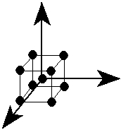
Many of you have seen my matrix of hypothesis testing methods. The
matrix is a two-way classification table of distribution
characteristics (mean, standard deviation, proportion, counts, and
distribution shape) and context/experiment design (one population,
paired samples, two populations, and many populations) that is used
to select analysis methods for different quality engineering
problems. We use the table by choosing a distribution characteristic
to be studied (a row in the table) and a context (a column in the
table). The intersection of the row and column lists the analysis
methods that are available. For example, if you want to compare the
means of two products or processes, the intersection of the mean row
and the two populations column suggests the following analysis
methods: two-sample t test, Tukey's quick test, boxplot slippage
tests, Mann-Whitney test. At this month's meeting we'll discuss the
use of this matrix and also where specialized quality engineering
methods like SPC, acceptance sampling, and tolerance intervals
belong.
Managing Missing Values in Designed Experiments
II, 6 June 2025, 7:30-9:00AM, by Zoom
At last month's QMN meeting we started discussing how to handle
missing values in a designed experiment. In that meeting we covered
how to detect missing values using the correlation matrix of model
terms and how missing values affect estimates for model
coefficients. At this follow-up meeting we will discuss specific
strategies to mitigate the effects of missing values.
Managing Missing Values in Designed Experiments,
2 May 2025, 7:30-9:00AM, by Zoom
When we build a designed experiment* we usually build an equal
number of runs (aka replicates) in each of the experiment's cells
because that imparts some desirable mathematical properties to the
model we build from the data. I was working recently with a customer
who chose runs for an experiment from historical data resulting in
an unequal number of runs/replicates in the cells of the experiment
design. He was correctly concerned about the effects of the
unbalanced design and asked for help with the analysis. At this
month's QMN meeting we'll look at how to use a correlation matrix to
detect unbalancedness in designed experiments, its consequences, and
some potential corrective actions for the analysis including the
following methods: ignoring the problem, omitting some runs, mean
substitution, and imputation methods for managing missing values.
* A designed experiment is any experiment that involves the planned
collection of data from a process for the purpose of understanding
that process better to aid in its management, improvement, or
control. The data set could be very simple (e.g. data collected for
a single response from a single stable population) or very
complicated (e.g. data collected for one or more responses from a
factorial, response surface, or other design).
Comparing Different Models In Designed
Experiments, 4 April 2025, 7:30-9:00AM, by Zoom
One of the things that we learn to do during the analysis of a
designed experiment is to fit a first, best guess model, and then to
refine the model, usually by dropping terms that are not
statistically significant. The goal of that process is to find the
simplest model that explains the data. But refined models aren't the
only family of alternative models to consider when fitting models to
a data set. Some of the cases that we will consider are:
When there are different research questions being considered,
different models might be required for the different research
questions.
In a complicated experiment design how can we answer the
question "Is there anything at all interesting happening?"
How do I fit a model to a balanced full factorial experiment
design when one or more complete cells of the experiment is
missing?
I designed my experiment in terms of quantitative process
input variables but an alternate system for defining the process
input variables might work better.
Analysis of Life/Survival Data When There Are No
Failures, 7:30-9:00AM, 7 March 2025, by Zoom
I was recently helping Matt B. analyze data from a life/survival
study. Matt was trying to compare two products - an old product and
a new product - for the purpose of showing that the new product is
at least as good as the old one. Both products have a target life
that has to be met with specified reliability and confidence values.
For the old product Matt tested 21 units to the life target and had
no failures. For the new product he tested 16 units to the life
target without failures and then continued testing on 8 of those to
three times the life target, again without failures. This analysis
is complicated by the fact that in reliability analysis the width of
confidence intervals for common reliability metrics is a function of
the number of units that failed - not the number of units that were
tested - and Matt had no failures of either product. At this month's
QMN meeting we'll discuss what analyses we can do with these data
and if we can answer the "at least as good as" claim.
A Checklist of Good and Bad Statistical Practices
(Part 3), 7:30-9:00AM, 7 February 2025, by Zoom
We spent the previous two QMN meetings reviewing my checklist of
good and bad statistical practices. I thought that we'd get through
the entire list in the first meeting, but you guys have had good
suggestions and questions and some of the items on the list have
involved some detailed discussions. At this month's meeting we'll do
a quick review of what we've previously covered and then cover the
last twenty or so items on the list. I have attached it in its
latest version so please try to review it in advance to see if you
have anything to add or any recommendations for changes.
A Checklist of Good and Bad Statistical Practices
(Part 2), 7:30-9:00AM, 10 January 2025, by Zoom
At last month's QMN meeting we started discussing a long list of
good and bad statistical practices that I developed for a new pharma
customer. The list was very well received and I have since added
much to it. At this month's meeting we will finish this discussion
by 1) reviewing items on the first half of the list and 2) covering
the items on the last half of the list. I've attached the document
so you can review it in advance.
A Checklist of Good and Bad Statistical Practices
(Part 1), 7:30-9:00AM, 6 December 2024, by Zoom
Some of my consulting friends and I recently did applied statistics
training for a new pharma customer who is expanding into a product
type where we have experience but they do not. The purpose of the
training was to identify and instruct them in the use of the FDA's
preferred statistical methods for this product type. The last
document that we presented at the end of three days of training was
a big hit with the students. The document was a list of about 80
potential issues with examples of good and bad practices. (I think
it was the bad practices that really resonated with the students.) I
know that you (i.e. QMN members) have much more experience with
these issues so I'd like your help refining and revising the
checklist.
Debugging the Real-Time Data Collection and Processing
Functions of a Hobby Electronics Project, 7:30-9:00AM, 1
November 2024 via Zoom
In the QMN meeting back on 5 August 2022 I described some of the
real-time data processing problems I was having on my hobby
electronics project to replace the instruments on my sailboat. At
that time I was focussed on fixing a distracting time lag problem
between when an event occurred and when it would appear on the
instrument display. I was using a simple exponentially-weighted
moving average (EWMA) filter which comes from SPC to smooth the
noisy data. A known down-side of the EWMA filter is that it
introduces a time lag in the response. I made the mistake of
attributing the time lag that I was observing to the EWMA filter so
I was investigating other filters with shorter time lags but
sufficient smoothing. This sailing season I discovered that the time
lag problem was coming from a combination of two different causes:
1) my code wasn't processing the data stream correctly and 2) the
Raspberry Pi computer I was using to process the data and display
the results wasn't fast enough for the job in its original
configuration. I was able to fix both problems and now the system
does an excellent job collecting, processing, and displaying data.
Paradoxes in Statistics, 7:30-9:00AM, 4 October
2024, by Zoom
Statistical methods can be confusing enough, but they are aggravated
by a set of common traps/mistakes that get clustered into a family
of "statistical paradoxes". (See the list in Wikipedia:
https://en.wikipedia.org/wiki/Category:Statistical_paradoxes.) With
training and practice you can learn how to recognize and avoid these
potential analysis errors. We'll consider some of these paradoxes at
this month's QMN meeting.
An Introduction to Blue Sky
Statistics Statistical Software, Sanjay Kumar, CEO, Blue Sky
Statistics, 7:30-9:00AM, 2 August 2024, by Zoom. Sanjay Kumar, CEO and co-founder of
BlueSky Statistics, a Chicago-based company, will introduce BlueSky
Statistics Software through a live demo and Q&A. BlueSky
Statistics is a comprehensive, easy-to-use, point-and-click
statistics and data analytics software to meet the needs of all
process and quality improvement initiatives (based on well-known
DMAIC methodology). The software is designed for quality engineers,
process improvement professionals, and Six Sigma practitioners of
all levels for a fraction of the cost compared to MINITAB, JMP, and
other expensive software licenses. The software has been used in
over 135 countries. Many organizations across industries have
switched to BlueSky Statistics from JMP, MINITAB, SPSS, and others.
Join the session to see a live demo of the important features such
as process capability analysis, measurement system analysis, SPC
charts, distribution fit analysis, hypothesis testing, regression
analysis, graphs and plots, DOE, and more as time permits.
Pugh Concept Selection Matrix, 7 June 2024,
7:30-9:00AM, by Zoom
Following the Analyze phase of the Six Sigma DMAIC process (for
improving an existing process) or the DMADV process (for designing a
new product or service) it is necessary to leverage the process
model developed in the Analyze phase to choose the best solution to
implement in the Improve or Design phase, respectively. Sometimes a
single solution will stand out and there are no questions about how
to proceed; however, when there are multiple competing candidate
solutions it will be necessary to select the best one. There are
many methods available (e.g. multi-voting) to assist in the solution
selection process but in particularly difficult situations a more
rigorous method like the Pugh Concept Selection Matrix method may be
required. This method uses a two-way classification matrix of
performance criteria versus candidate solutions and scoring relative
to a standard solution to identify the best of the candidate
solutions.
Acronyms:
DMAIC Define, Measure, Analyze, Improve, and Control
DMADV Define, Measure, Analyze, Design, Verify
The Ramirez-Runger Test: Do my data come from a
single stable population?, 3 May 2024, 7:30-9:00AM, by Zoom
When we're collecting data from some process, we usually make the
assumption that the process is stable in time, that is, that its
distribution location, variation, and shape are all constant. If a
process is not stable in time then we can't expect to fit a
distribution model to the data. We need a method to discriminate
between stable and unstable processes.
We often test for the stability of a process by inspecting a run
chart of the data; however, this method is subjective and may not
detect subtle problems so we need a more discriminating test. Enter
the Ramirez-Runger test. I only learned about this test recently
from a Quality Digest article by Don Wheeler (link below) and the
test has only been around since 2006 so it doesn't appear in any of
my archaic reference materials.
The Ramirez-Runger test works by comparing two measures of the
process variation using an F test for two standard deviations. The
first of the two measures is simply the standard deviation of all of
the sample data. The second measure is the standard deviation
estimated from the moving ranges where moving ranges are the
absolute values of the differences between consecutive observations.
If the data come from a time stable process, then the two standard
deviation estimates should be comparable to each other. If the data
don't come from a time stable process, then the two standard
deviation estimates will diverge and we can't expect to fit a
distribution to the data. I'm planning to adopt this test in my
process capability study protocol and other procedures that require
the stability assumption.
Wheeler,
https://www.qualitydigest.com/inside/lean-article/test-use-all-other-tests-040324.html
Ramirez and Runger, Quantitative Techniques to Evaluate Process
Stability, June 2006, Quality Engineering 18(1):53-68
The Many Uses of the Sign Test, 5 April 2024,
7:30-9:00AM, by Zoom
The nonparametric sign test is one of the few statistical methods
that have a simple instinctive interpretation. It appears any time
you're expecting binary observations to have a 50/50 split. Consider
what is perhaps its best known example:
A balanced coin is tossed 10 times. How would you
feel if the coin delivered 5 heads and 5 tails? 4 heads and 6 tails?
3 heads and 7 tails? ...
Hopefully you can see where this is going. At some point, certainly
for a 1/9 or 0/10 split, you would get suspicious and check the coin
to see if there is any evidence against the "balanced" claim.
When binary observations, like the heads or tails results in the
coin toss example, are coded as plus (+) and minus (-) signs, then
we just have to count the experimental number of plus and minus
signs and test for significance using the "sign test". The number of
heads x in n trials under the null hypothesis that the coin is
balanced (p = 0.50) follows the binomial distribution b(x;n,p =
0.50). Knowledge of this distribution allows us to determine the
statistical significance of the data.
At first the scope of problems where you would expect the sign test
to be appropriate might seem pretty narrow; however, it turns up in
a lot of places:
One-sample sign test for location
Paired-sample sign test for location
Paired-sample test for proportion (McNemar's test)
Cochran's test for trend (as in linear regression)
Regression lack-of-fit test
The sign test is usually not the most powerful test method
available, but it is so simple to learn and easy to apply that it is
invaluable as an exploratory or quick test. With some practice
you'll learn to recognize the many places that it appears and how to
interpret its results.
Accelerated Life Test of a Hand Sanitizer
Product, 2 February 2024, 7:30-9:00AM, by Zoom
In our December and January meetings we discussed many ways to
analyze the data for an accelerated life test. This month we'll
consider another type of life test. In the previous discussions, the
life response was measured in hours or cycles to failure with the
possibility of right censoring. This month we will consider the
determination of the shelf life for a biomedical hand sanitizer
product that must comply to FDA Guidance Document ICH Q1E Evaluation
of Stability Data. The product's response that determines its shelf
life is the chemical concentration of its sanitizing active
ingredient. The concentration is high at the time of manufacture but
decays slowly over time approaching the concentration's lower spec
limit. ICH Q1E specifies the shelf life-determining condition and
allows for both real time room temperature and temperature
accelerated testing. We'll show that by evaluating samples stored at
25 and 40C it is possible to demonstrate a two year shelf life claim
using 6 month data.
Design, Analysis, and Sample Size Calculations
for an Accelerated Life Test - Part 2, 5 January 2024,
7:30-9:00AM, by Zoom
We didn't finish our discussion of accelerated life tests last month
so we will continue our discussion in January. See the December
abstract for the planned scope of the discussion.
Design, Analysis, and Sample Size Calculations
for an Accelerated Life Test, 1 December 2023, 7:30-9:00AM, by
Zoom
I am working on an experiment design and sample size calculation for
an accelerated life test for a customer. MINITAB has methods for the
the data analysis and the sample size calculation; however, I'm
having difficulty configuring the sample size calculation menu. I
thought that I would talk through these issues at this month's
meeting. The abstract from our last discussion on this topic (minus
the sample size calculation) is here:
Use Accelerated Testing to Reduce the Length of Life
Tests (5 May 2017)
In an ordinary life test, where the response (such as the fraction
of units surviving or the concentration of a chemical) changes
with time, the units under test are operated at the same
conditions as are expected in actual use until they reach a
defined end-of-useful-life condition. The downside of this
approach is that if the life of the product is expected to be very
long then the duration of your life test will also need to be that
long. And iterations of the design could result in several
consecutive life test cycles that will surely exceed the limits of
any manager's patience. Thankfully the duration of many life tests
can be reduced by operating the units under test at a higher
stress level than they would see in normal use, thereby
accelerating the rate of change of the response. Common stress
variables are temperature, pressure, and voltage. Through careful
design of the life test experiment - with particular attention
paid to resolving the effect of the accelerating variable - we can
build a model for the life test response that allows us to make
life predictions for normal operating conditions from the
accelerated life test data. This approach can reduce the duration
of a life test to just a fraction of the time it would take to
perform the same test under unaccelerated conditions.
Goodness of Fit Tests for Linear Regression, 3
November 2023, 7:30-9:00AM, by Zoom
One of the assumptions of the linear regression method is that the
form of the model is appropriate for the data. This condition is
referred to as "goodness of fit" or "lack of fit". Many people make
the mistake of assuming that goodness of fit is indicated by the
R-squared metric; however, R-squared and goodness of fit address
different issues so other methods of assessing goodness of fit are
necessary.
The easiest way to assess whether a model fits the data is to create
a plot showing the model superimposed on the data. If the model
tracks the data well then we probably have a good fit. This
assessment "by eye" works well but it can be insufficient when
subtle discrepancies are present or the model is too complicated to
display in graphical form. In these cases formal quantitative
goodness of fit tests are required. At this week's QMN meeting we
will consider some of these goodness of fit tests and implement them
manually and using MINITAB's built in capabilities.
Examples of Equivalence, Superiority, and Noninferiority
Tests, 6 October 2023, 7:30-9:00AM via Zoom
At last month's QMN meeting we discussed the formulation of
equivalence, superiority, and noninferiority test hypotheses. We'll
continue that topic this month by discussing detailed examples of
these cases. If you've run any of these tests yourself, please
consider volunteering to explain your work.
Formulating Equivalence, Superiority, and
Noninferiority Test Hypotheses, 1 September 2023, 7:30-9:00AM,
by Zoom
After learning the basic significance test methods we often find
ourselves with the need to perform equivalence, superiority, and
noninferiority tests. The analyses and interpretation of these
methods borrow heavily from significance testing but they introduce
new issues that complicate their formulation. We'll consider these
issues at September's QMN meeting.
Sample Size Calculations for One-way, Two-way,
and Multi-way Classification Designs, 4 August 2023,
7:30-9:00AM, by Zoom
In our previous sessions we discussed how to adapt the sample size
calculation for the two-sample t test using Bonferroni's correction
to the more general case of testing for biases between three or more
treatment groups in one-way and multi-way classification designs;
however, we never looked at the exact sample size calculation
methods for those designs. In this month's meeting we will start
with the sample size calculation method for F tests for two-way and
multi-way classification designs and then compare their results to
those from the Bonferroni-corrected two-sample t test method.
Connections Between Sample Size Calculations for
the Two-sample T Test, Two-level Factorial Designs, and Linear
Regression, 2 June 2023, 7:30-9:00AM, by Zoom
In recent past QMN meetings we've discussed sample size calculations
for the two-sample t test, the two-level factorial designs, and
linear regression. All sample size calculations have similar
structure, but these three methods have particularly close
relationships that deserve to be discussed in more detail. The
benefit of understanding these relationships is that it can make it
easier to choose the necessary inputs for the calculations and there
may be opportunities to perform a calculation for one method by
using another method's solution or software implementation.
Sample Size Calculations for Linear Regression, 5
May 2023, 7:30-9:00AM, by Zoom
The next topic in our ongoing discussion of sample size calculation
methods is linear regression. This is probably one of the most
abused and ignored sample size calculation methods in engineering,
science, business, and industry. Proper consideration of sample size
for linear regression must take into account the goal of the
experiment - usually to quantify (with a confidence interval) or
test the value of (with a hypothesis test) the slope of the
regression line; however, there are other crucial inputs to the
problem including the range of observations on the independent
variable (i.e. x) scale and the distribution of observations over
that range. Given all of these inputs and an estimate for the
noise/repeatability of the response (i.e. y) variable, an objective
sample size can be determined for the experiment to build a
regression model. These calculation methods are relatively simple;
however, they are not supported in MINITAB and other common
software.
Sample Size Calculations: Poisson Count
Responses, 7:30-9:00AM, Friday, 7 April 2023, by Zoom
At this month's QMN meeting we will discuss sample size calculations
for Poisson count responses. Poisson counts appear whenever you are
counting the number of events per unit area of opportunity, such as:
Number of military officers killed by horse kicks per year
(this problem was the origin of the Poisson distribution)
Defects per sampling unit (e.g. an SPC defects chart)
Paint defects per car door
Radioactivity counts per second (e.g. Geiger counter)
Phone calls per day
Defects per submission of a form, e.g. purchase order or
invoice
Number of accidents per year (for an organization, e.g.
amusement park)
Number of bank failures per year
Number of people waiting in line at the checkout counter
We will consider sample size calculations for Poisson counts for the
following situations:
Confidence interval for the Poisson mean (one sample)
Hypothesis test for the Poisson mean (one sample)
Confidence interval for the difference between two Poisson
means (two samples)
Hypothesis test for a difference between two Poisson means
(two samples)
Hypothesis test for differences among many Poisson means
(analogous to ANOVA)
Thankfully MINITAB supports most of these methods.
Sample Size Calculations: Two Proportions,
7:30-9:00AM, 3 March 2023 by Zoom
One of the most common and important experiment design categories is
the two populations design. This design can be used to generically
compare any two populations but it is especially important when
comparing a gold standard or "control" method to a competing test
method. This test versus control design has the benefit that it
considers the test and control methods under the same conditions
compared to the relative weakness of evaluating a test method in a
one sample test without direct comparison to the control. The two
populations design can be applied to measurement and attribute
responses.
When the observed response in a two populations design is a binomial
count, such as when we count the number of pass/fail events observed
in a predetermined number of trials, then the statistical analysis
is done using a two proportions test. There are two such tests
available: Fisher's Exact Test and a normal approximation test.
Fisher's test works under all circumstances but the calculations can
be difficult. The normal approximation method is applicable under
some common conditions and is easier to apply. Both analysis methods
are implemented in good statistical software, such as in MINITAB's Stat>
Basic Statistics> 2 Proportions menu.
As with all data collection and analysis exercises for the purpose
of studying or improving a process, the two populations study
deserves to be preceded with a sample size calculation to get the
sample size correct. An uninformed choice of sample size runs the
risk of 1) being too large and wasting time and resources or 2)
being too small risking an incorrect decision. Given appropriate
inputs about the history of the processes under study and the goals
of the experiment, an objective sample size can be calculated.
MINITAB provides support for those cases that can be analyzed using
the normal approximation method with its Stat> Power and
Sample Size> 2 Proportions method. When the normal
approximation conditions aren't satisfied the custom FishersPower.mac
MINITAB macro can be used. At this month's QMN meeting will consider
both of these tools.
Sample Size Calculations: One Proportion,
7:30-9:00AM, 3 February 2023 by Zoom
Near the top of the list on the Pareto chart of most-used
statistical analysis methods are methods for one proportion. These
methods include the generic confidence intervals and hypotheses
tests for one proportion but they also include specialized quality
engineering applications such as attribute acceptance sampling and
reliability demonstration tests. At this month's QMN meeting we will
look at sample size calculations for the following one-sample
proportion goals:
Demonstrate that the proportion defective is less than a
specified value
Demonstrate that the reliability is greater than a specific
value
Quantify a proportion with a two-sided confidence interval
Reject a claimed value of a proportion in favor of an
alternative proportion
Thankfully MINITAB provides support for all of these methods but you
can also perform these calculations with Russ Lenth's free Piface
sample size calculator (https://homepage.divms.uiowa.edu/~rlenth/Power/)
if you don't have MINITAB.
Sample Size Calculations: Standard Deviations and
Process Capability, 7:30-9:00AM, 6 January 2023 by Zoom
At our December meeting we discussed sample size calculations for
the two-sample means problem and the associated many-sample means
problem. At our January QMN meeting we will discuss sample size
calculations for standard deviations and MINITAB's support for the
method. We will also study how those methods can be adapted for
sample size calculations for process capability metrics. The result
is quite depressing.
An Introduction to Sample Size Calculations -
Part 3, 7:30-9:00AM, 2 December 2022, by Zoom
At our November meeting we discussed sample size calculations for
the one-sample and two-sample Student t tests for location and at
the end of that discussion we rushed into the extension of the
two-sample t test to many samples. This month we'll go back and take
the sample size calculation for the many-samples case more slowly.
We'll review the sample size calculation for the two-sample t test,
we'll extend its scope to many samples using Bonferroni's
correction, and then we'll compare that result to the sample size
for one-way ANOVA. We'll also look at how the sample size
calculation for one-way ANOVA relates to ANOVA for two-way and
multi-way classification designs.
An Introduction to Sample Size Calculations -
Part 2, 7:30-9:00AM, 4 November 2022, by Zoom
At last month's meeting we started a discussion of sample size
calculation methods. We started all the way back at the beginning of
the topic and took our time with the material. We got through the z-
and t-based one-sample tests and confidence intervals for the
population mean - less than I'd planned but that's a good thing.
This month we'll review those methods and then continue on with the
two-sample test and confidence interval for the difference between
two population means. We'll also extend the solution for the
two-sample case to three or more samples. I plan to go over this
material as slowly as you like, so please come prepared to ask lots
of questions. We will continue with this topic in future meetings.
An Introduction to Sample Size Calculations,
7:30-9:00AM, 7 October 2022, by Zoom
We frequently address the topic of sample size calculations in this
forum, usually taking on a specific method of interest. I recently
heard a request to backtrack from the advanced material a bit and
take the topic from the very beginning, so at the October QMN
meeting we will discuss the sample size calculations for a few of
the most basic statistical analyses:
Confidence interval for a population mean
Hypothesis test for a population mean
Confidence interval for the difference between two population
means
Hypothesis test for a difference between two population means
One-sided upper confidence limit for the population proportion
defective
One-sided hypothesis test for the population proportion
defective
I plan to go over this material as slowly as you like so please come
prepared to ask lots of questions. We can continue on with this
topic in future meetings.
Diagnostic Tests and ROC Curves, 7:30-9:00AM, 2
September 2022, by Zoom
A diagnostic test is used to distinguish two populations, for
example, between diseased and healthy subjects, using a quantitative
measurement compared to a threshold value. Observations that fall on
one side of the threshold are judged to have the disease and
observations that fall on the other side of the threshold are judged
to be healthy. Diagnostic tests are also common in engineering,
manufacturing, and other non-medical situations.
When the tails of the distributions of diseased and healthy subjects
overlap on the measurement scale, the diagnostic test will
misclassify some of the subjects. For example, the test will produce
some false positives (subjects who are healthy but whose test
indicates that they have the disease) and false negatives (subjects
who have the disease but whose test indicates that they are
healthy). Both types of errors have associated costs that must be
taken into account when choosing the threshold value.
The overall performance of a diagnostic test is evaluated in terms
of its true negative rate or specificity (the fraction of healthy
subjects who are classified correctly) and its true positive rate or
sensitivity (the fraction of diseased subjects who are classified
correctly). The trade-offs associated with different threshold
values can be evaluated using a receiver operating characteristic
(ROC) curve - a plot of the true positive rate or sensitivity versus
the false positive rate or 1 - specificity.
Smoothing Noisy Time Series Data - A Solution
from the Technical Trading Stock Market Community, 7:30-9:00AM,
5 August 2022, by Zoom
Most of you know that my wife and I have a sailboat that we race and
cruise on Lake Erie. The boat's instrument system is over 20 years
old now and its LCD displays have lost their contrast so are
effectively useless. I could/should just replace the instrument
system but where is the fun in that? The boat speed, depth, and wind
sensors all still work great, so as a hobby electronics project I
set out to re-use the sensors and build everything else from
scratch. I'm using an Arduino-like microcontroller to read the raw
instrument data and a Raspberry Pi to process the data and write
responses to a waterproof sunlight readable touchscreen display.
Needless to say, there have been a lot of stumbling points along the
way - little things like learning Arduino, Raspberry Pi, Python, and
Kivy. I've learned a lot though so I keep telling myself that this
is fun.
At this point all of the basic functionality of the system is
working but I have encountered another unexpected stumbling point: I
expected the sensor data to be noisy but assumed that filtering out
the noise in software would be easy. NOT! My early filtering
attempts came from simple statistical methods for time series data.
Those methods do successfully filter the data but introduce a long,
unnerving, distracting delay between a sudden change on the boat
(such as wind speed) and when the effect of that change shows up on
the displays. I knew there would be a trade off between the degree
of smoothing and the time lag but I haven't able to find an
acceptable compromise. I had to find a better way to filter the data
without introducing long time lags. I initially looked to the
electronics community for a solution but was surprised to find that
the solutions I needed come from "technical" stock market trading.
Technical traders write algorithms to identify reliable patterns in
stock market data and then buy and sell stocks on that basis.
Recognizing a change in a process quickly and reliably is crucial to
their success. Many of the most successful methods are proprietary
but the basic methods are well known and implemented in commonly
available trading software. At this month's QMN meeting I will
describe some of the time series filtering methods that I've
discovered. The basic methods are native in MINITAB but I'll
describe some other simple algorithms that can be implemented in
MINITAB code or other software.
The Rank-Order Transform and Nonparametric
Analysis Methods for When Your Data Aren't Normal, 3 June 2022,
7:30-9:00AM, by Zoom
We all know that the classical statistical analysis methods like the
one-sample t test, two-sample t test, and ANOVA require that the
data be normally distributed. Those methods aren't particularly
sensitive to deviations from normality, especially when the sample
sizes are large (yeah Central Limit Theorem!), but when you're not
sure if a deviation from normality is too much then robust
alternatives to the classical methods are provided by analogous
nonparametric ones. The nonparametric methods (for the three tests
mentioned) involve rank transforming the observations - that is,
replacing the original measurement values with their rank order. The
analogous nonparametric analysis methods for rank ordered data are
provided by the one-sample Wilcoxon test, the Mann-Whitney test, and
the Kruskal-Wallis test. MINITAB supports all of these methods from
its Stat> Nonparametrics menu. Also remember that the
nonparametric methods can be applied to any rank ordered data, even
when a measurement scale isn't available.
Fitting Multiple Regression Models with Inputs
Expressed in Physical Units, 7:30-9:00AM, 6 May 2022, by Zoom
When we build a designed experiment in MINITAB, MINITAB prompts us
to enter the physical values of our process input variables (PIV);
however, when it reports the results of the analysis it expresses
the PIVs in coded units. For example, we might specify Temperature
as a PIV with physical levels 30 and 50C, but MINITAB recodes those
levels to -1 and +1, respectively, when it reports the regression
equation. Why does it do that? Why doesn't it just report the
regression equation in physical units? This seeming quirk isn't
unique to MINITAB either. Every other reputable statistical software
does the same thing. The need to "code" the PIVs to +/-1 values (or
some other coding scheme) is required to determine independent and
accurate regression coefficients that can be used to judge the
effect of and the statistical significance of the PIVs. A regression
equation CAN be expressed in terms of the physical units; however,
those regression coefficients may be contaminated with contributions
from other PIVs that will lead to confusion and misinterpretation of
the effects of the PIVs on the response. Proper coding of the PIVs
solves that problem. At this month's QMN meeting we will look at the
root cause of the need to code PIVs when doing multiple regression
and we will identify the properties of models that permit or don't
permit expressing a multiple regression model in terms of the
physical values of the PIVs.
Double and Multiple Sampling Plans Versus
Bonferroni-Corrected Single Sampling Plans Adapted for Double
and Multiple Sampling, 1 April 2022, 7:30-9:00AM, by Zoom
At our last meeting I described how to use Bonferroni's method to
expand a zero acceptance number sampling plan to allow one or more
defectives in double or multiple inspection episodes. The Bonferroni
method is technically valid; however, it overlooks a structural
issue in adapting single sampling plans into double or multiple
sampling plans that makes its sample sizes larger - sometimes much
larger - than they need to be. At this month's meeting we will
compare the Bonferroni-corected single sampling plans adapted for
double and multiple sampling to the formal methods available for
designing double and multiple sampling plans.
Use of Bonferroni's Method to Account for Early
Defectives in Attribute Sampling, 7:30-9:00AM, 4 March 2022, by
Zoom
At last month's QMN meeting we discussed the application of
Bonferroni's correction to the post-ANOVA multiple comparisons test
problem; however, applications of Bonferroni's method have much
broader applications. I was recently helping a customer design a
single sampling plan for attributes to demonstrate that the
proportion defective of a process is less than 5% with 95%
confidence. The required sample size for the zero acceptance number
sampling plan comes from the well known Rule of 3: n = 3/pmax where
pmax is the allowed upper limit on the proportion defective. To meet
the 95% confidence of less than 5% defectives goal, the required
sample size is n = 3/0.05 = 60. But my customer was rightly
concerned about the possibility of finding a defective unit before
reaching the n = 60 sample size so we revised the sampling plan
design using Bonferroni's method to allow a two-stage sampling
process that allows for an early defective. The nature of this
problem is also present in interim analysis and double sampling
plans. We'll look at the applications of Bonferroni's method in
sampling plan design and these related methods at this month's QMN
meeting.
Bonferroni's Correction for Multiple Comparisons
Tests, 7:30-9:00AM, 4 February 2022, by Zoom
When we're planning a statistical analysis by hypothesis test or
confidence interval one of the decisions we have to make is what
type 1 or false alarm error rate to tolerate. The most common choice
is 5%; however, that choice must be reconsidered when more than one
test is planned. This problem arises naturally and is very common.
For example, if we need to test for a difference between two
treatment groups then only one test is necessary and a 5% error rate
is appropriate, but if there are more than two treatment groups then
we will have to test for differences between all possible pairs of
treatments and the number of tests can grow very large. For example,
in the simple case of tests to compare five treatment groups there
will be 10 tests: 12, 13, 14, 15, 23, 24, 25, 34, 35, and 45 where
the numbers 1, 2, ..., 5 indicate treatment group IDs and a pair of
numbers indicates a test between those treatments. The large number
of tests, each with a 5% error rate, makes it more likely that we
will commit one or more errors among the many tests required. This
forces us to reconsider the choice of a 5% error rate per test. The
first solution to deal with this multiple comparisons testing
problem was offered by Bonferroni who observed that we can control
the error rate for a family of tests by setting the individual test
error rate equal to the family error rate divided by the number of
tests we intend to perform. In our previous example of 10 tests to
compare five treatment groups, Bonferroni's method advises that to
hold a 5% error rate for the family of 10 tests we need to use a
0.05/10 = 0.005 or 0.5% error rate for individual tests. This
approach is simple, conservative, and very flexible so it is used
more often than every other type of multiple comparisons test.
Weighted ANOVA and Weighted Regression (What To
Do When You Can't Find a Variable Transform), 7:30-9:00AM, 7
January 2022, by Zoom
When we perform ANOVA or regression we always analyze the model
residuals to determine if the assumptions of normality and
homoscedasticity (aka equal variances) are satisfied. When they're
not, a variable transform - such as taking the log, square root,
power function, or reciprocal of the response - may resolve the
problem and we can go on with our planned analysis. However, there
are times when the residuals are heteroscedastic and we just can't
find a variable transform that fixes the problem. A common example
is when the experimental data are collected using two or more
different measurement instruments or methods that have different
inherent measurement precision. ANOVA and regression fail under
these conditions; however, they can be salvaged by proper weighting
of the residuals. This sounds complicated but it's quite simple:
weighted ANOVA or regression requires you to identify a function
that accounts for the differences in standard deviations, use the
function to determine weights, and then re-run the ANOVA or
regression with the weights incorporated into the model. We can even
use the original residuals diagnostic methods for checking
assumptions by analyzing the weighted residuals instead of the
original/raw residuals. We'll take a look at these methods in this
month's meeting.
Resampling Methods, 7:30-9:00AM, 3 December 2021,
by Zoom
I'm so used to my old habits when working in MINITAB that I often
don't notice additions that have been made to the program. Recently
I was talking a customer through an analysis and did a double-take
when I noticed the Calc> Resampling menu. I'm not sure
when this menu was added, but it's a great addition to MINITAB and
definitely worth talking about in a QMN session.
The traditional methods for constructing confidence intervals and
performing hypothesis tests are based on the z, t, chi-square, F,
and other distributions that can feel abstract and, frankly, much
like magic to novices. Even after we get those methods under control
there are often situations in which we can be uncertain or
uncomfortable that the assumptions required for their use are
satisfied. In such circumstances, the family of resampling methods,
which rely only on sample data and special but intuitive resampling
procedures, can provide a comforting and useful alternative set of
analysis tools that have fewer assumptions and constraints than the
traditional methods. So at this month's QMN meeting we will discuss
the use of resampling methods for confidence intervals and
hypothesis tests and compare their results to those from the
traditional methods. This topic is likely to span more than one
session so make sure you join us next week so that you're not behind
in the following sessions.
Tests and Sample Size Calculations for Poisson
Count Responses, 7:30-9:00AM, 5 November 2021, by Zoom
We've spent a lot of time discussing tests and sample size
calculations for measurement responses and for proportions (e.g.
proportions defective or yield); however, we haven't taken up the
topic of tests and sample size calculations for Poisson distributed
counts, such as defect counts or pretty much any
count-per-unit-something. At this month's QMN meeting we will
discuss the one-sample, two-sample, and many-sample tests for
Poisson counts and their associated sample size calculations.
Tests for Homoscedasticity (aka Equal Variances)
by F, Bonett, and Levene Test Methods, 7:30-9:00AM, 1 October
2021, by Zoom
At this month's QMN meeting we will review the F test for
homoscedasticity and consider two alternative tests: Bonett's and
Levene's tests.
One of the most frequently checked assumptions when working with two
or more independent populations is the assumption of equal variances
or homoscedasticity (from the Greek for "same dispersion"). In the
simplest case of two treatment groups, the classical method for
testing the homoscedasticity assumption is the F test where the F
statistic is given by the ratio of the two sample variances. The F
test works very well when the two populations being studied are
normally distributed; however, errors creep in when those
distributions deviation from normality. This issue is sufficiently
serious that modern versions of MINITAB default to more robust
methods (Bonett and Levene) and bury the F test in its submenus.
Levene's method also has the added benefit of being applicable when
there are two, three, or more treatment groups.
The Two-Sample T Test and the Paired-Sample T Test,
7:30-9:00AM, 3 September 2021 by Zoom
Two of the most frequently used hypothesis testing methods are the
two-sample t test and the paired-sample t test. Both methods are
tests of means so they're obviously closely related which makes them
easily confused but they deal with very specific situations and it's
crucial to choose the correct method for an analysis
The two-sample t test is applied when the two samples are
drawn from independent populations.
The paired-sample t test is used for paired observations
taken on the same physical units to test for a difference caused
by the variable that distinguishes the observations in the
pairs.
Example 1. Suppose that you need to test for a difference in the
operating lifetime of a device on batteries supplied by two
different manufacturers. To perform the experiment you would collect
random samples from the two manufacturers, operate the device on
those samples and record the battery lifetimes, and then use the
two-sample t test to determine if they are different from each
other.
Example 2. Suppose that you need to test for a difference between
two nondestuctive test methods that are supposed to deliver the same
results. To perform the experiment you would collect a sample of
units to be tested, measure them under both test methods, and then
use the paired-sample t test to determine if there is a bias between
the two test methods.
This all sounds pretty simple; however, it's not always so easy. I
was recently working on a complicated test plan for a customer. We
designed the experiment and I immediately recognized the opportunity
for using the two-sample t test; however, I failed to recognize that
the data collection scheme also provided the opportunity for using
the paired-sample t test. I was uncomfortable with the two-sample t
test analysis that I recommended and eventually considered a
simplified version of the experiment that revealed the paired-sample
t test opportunity. As it turned out, the paired-sample t test
required a smaller sample size than the two-sample t test, so the
extra sample size that we planned for the two-sample t test just
provides greater power for the paired-sample t test.
Organizational Statistical Maturity Checklist, 7:30-9:00AM,
6 August 2021 by Zoom
As a consultant I see a wide range of statistical and quality
engineering skills and practices among my many customers. Invariably
they all want to know how their company compares to others. An
appropriate instrument or measurement tool to make such comparisons
is an organizational statistical maturity checklist. I started such
a checklist long ago intending to get back to it some day and now is
the time. At this month's QMN meeting I'll present my draft and
notes on the topic. Please join our discussion to contribute your
own thoughts on what should be included in the checklist, how it
should be organized, and how it should be scored. Maybe we'll follow
up by executing the checklist at work and then comparing results at
a future meeting.
Modeling Standard Deviations, 7:30-9:00AM, 4 June 2021 by Zoom
When we're doing experimental work our first concern is for
understanding how process input variables (PIV) affect the process's
mean response. The statistical analysis methods used to compare two
or more means or many means under diverse conditions are the
two-sample t test, ANOVA, and regression. There is an assumption
required of those methods that the standard deviation of the noise
in the process is constant under all conditions - a state referred
to as homoscedasticity. When that condition is not satisfied (i.e.
when the noise is heteroscedastic) we can often deal with the
problem by applying an appropriate variable transform to the
response. A logarithmic transform (log or ln) usually works. The are
times, however, when such transforms fail and it becomes necessary
to build experiments to study how the standard deviation of a
process's response changes as a function of the PIVs. These analyses
for standard deviations are performed using methods that are
analogous to those used for analyzing means. At this month's meeting
we will consider the tests and analysis methods available to study
how standard deviations vary in the context of experiments with two
treatment groups, many treatment groups, and in designed
experiments.
The Slipped Confidence Intervals Method versus
the Two-Sample t Test Method, 7:30-9:00AM, 7 May 2021, by Zoom
My friend Mark is planning a clinical trial for which we designed an
appropriate experiment to be analyzed using a two-sample t test with
a matching sample size calculation; however, his sponsors, who have
limited statistical knowledge and skills, were confused by how
"statistical power" enters the sample size calculation and have
demanded that we perform the analysis by the slipped confidence
intervals method instead. In this method, the data from two
independent populations are collected and confidence intervals are
calculated for their population means. If the two confidence
intervals are slipped, i.e. don't overlap, then we reject the null
hypothesis H0: the two population means are equal in
favor of the alternate hypothesis HA: the two population means
are different. While this analysis method is simple - it
certainly has a very easy-to-understand graphical presentation - it
suffers from some serious flaws that discourage its use. I learned
to avoid the slipped confidence intervals method long ago, but until
now I was never forced to look into it seriously. So this week we
will compare the wrong way to do the analysis (the slipped
confidence intervals method) to the right way to do the analysis
(the two-sample t test method).
Follow-up: After our discussion in this meeting we figured out that
when the confidence levels of the two confidence intervals is
adjusted to 84% the slipped confidence intervals method has Type 1
error rate of 5% and matches the statistical power of the two-sample
t test. That is, the two slipped confidence intervals test methods
using 84% confidence intervals is equivalent to the two-sample t
test.
Normality - When Does It Matter and When Does It
Not? (Part 3), 7:30-9:00AM, 2 April 2021, by Zoom
At the last two QMN meetings we've been talking about where the
normality assumption applies and where it does not, especially in
the context of process capability analysis. We weren't quite done
with that conversation so we're going to take it up again in this
third - and hopefully last - session on this topic. I'll come to the
meeting with a collection of examples that demonstrate the
difficulties that we've been having to prime the discussion.
Hopefully after this meeting we can achieve some better
understanding if not clarity on these issues.
Normality - When Does It Matter and When Does It
Not? (Part 2), 7:30-9:00AM, 5 March 2021, by Zoom
Many statistical analysis methods require or work better when the
data follow a normal distribution; however, in experiments with
complex structure it can be difficult to decide what to check for
normality. One example that we talked about last month - one that
instigated this discussion topic - is the very important problem of
process capability analysis when the data set contains samples from
several lots when there are biases between lots. There are three
distributions that could be tested for normality: the distribution
of the original data set, the distribution of the noise within lots,
and the distribution of the biases between lots. At this month's
meeting we'll discuss how to run the analysis in this situation and
some more complex ones.
Normality - When Does It Matter and When Does It
Not?, 7:30-9:00AM, 5 February 2021, by Zoom
I ran into two recent instances of mistakes made in testing for
normality to support another analysis:
My friend J is wrapping up his PhD and got into a disagreement
with his thesis advisor about the normality assumption in linear
regression for y = f(x). His advisor maintained that the
normality requirement applies to the y values; however, the y
values can do anything they want. It's the residuals in the y(x)
model that must be normal. (This mistake is even perpetuated in
Excel's Analysis> Regression add-in which produces the wrong
normal plot.) J went to his thesis defense with his advisor's
incorrect interpretation of the normality requirement in his
slide deck but the correct back-up analysis ready to go.
My friend S was analyzing a process capability study and found
strong evidence that his data weren't normal. When we looked
more closely we saw that the data set spanned many material lots
and that there were biases between the lots. The normality tests
were reacting to the clustering of observations caused by those
biases. We used ANOVA to separate the noise within lots from the
biases between lots and when we studied those distributions
separately they were both normal. The mash-up of two normal
distributions is also normal so even though S's raw data weren't
normal the underlying distributions were so we could continue on
with our process capability analysis using methods for normal
distributions.
These are just two of many possible ways that a simple normality
test is inappropriate and may mislead you. We'll talk about these
two and many other cases at this month's meeting.
Development, Validation, and Use of Subjective
Measurement/Observation Scales Using Ordinal Data, 7:30-9:00AM,
8 January 2021, by Zoom Way back at our 4 August 2017 QMN meeting we discussed
the development of a pseudo-measurement system for making subjective
observations on an ordinal scale. The specific application was Joe
R's need for developing a measurement system for interpreting the
severity of material corrosion. Ordinal scales have a sense of size
(e.g. this is bigger than that) but don't have a fixed unit of
measurement (e.g. inches, seconds, ...). Generally when presented
with an inspection made on a subjective ordinal scale we try to
upgrade the ordinal observations to a true quantitative interval
scale; however, there are many situations in which the upgrade is
impossible and we must live with the subjective ordinal data. When
this problem comes up we talk about it in the context of solving a
specific problem (like Joe R's in that QMN meeting); however, at
this month's QMN meeting let's talk about the general steps required
to develop, validate, and use measurements made on an ordinal scale.
We'll also talk about designing experiments for use with an ordinal
response and the associated issue of determining the sample size for
such an experiment.
Quality, Statistics, Engineering, and Science
Reading List, 7:30-9:00AM, Friday, 4 December 2020, by Zoom
On the small chance that anyone else out there still reads (yes, I
still read actual physical books with paper pages), let's discuss
our favorite quality engineering, statistics, engineering, and
science books. I keep a list of the books that I frequently
recommend posted here
that we can start from but come ready with your own recommendations.
Why We Randomize, 7:30-9:00AM, 6 November
2020, by Zoom
One of the good indicators of you or your organization's
"statistical maturity" is your understanding and insistence on the
use of randomization when you're collecting experimental data. As is
often the case, this discussion topic was instigated by a recent
customer experience. This customer performed a simple experiment to
compare four different treatment groups for possible differences in
their means and standard deviations and asked for my help in running
the analysis. (I wasn't involved in the design of the experiment at
all.) When I ran the analysis, which indicated the presence of
statistically significant differences between the treatment groups,
I included a disclaimer that because the run order of the
observations was not reported to me I couldn't say for certain
whether the observed differences were truly due to the treatment
groups or if they were due to an unobserved lurking variable if the
observations were not run in random order. Initially my customer
didn't notice or comment on my disclaimer, but when they looked at
the differences between the treatment groups those differences were
completely contradictory to what they expected but correlated well
with the non-random run order that they used to collect the data.
The experiment was expensive and time consuming to perform; however,
they can't deny that the observed effects are better explained by a
run order effect than by differences between the treatment groups so
they are reluctantly committing to repeat the experiment, this time
using a randomization plan to control for lurking variables and run
order effects. Lessons like this are hard to learn. Instructors and
advisors and technical experts can tell you again and again and
again that you should be randomizing but until you get burned in a
major, traumatic way, you never really understand or appreciate the
necessity of randomizing the order of the runs in your experimental
work.
Configuring MINITAB's Stat> ANOVA> General
Linear Model Menu (Part 2) and Related Methods,
7:30-9:00AM, 2 October 2020, by Zoom
Last month we discussed how to configure MINITAB's Stat>
ANOVA> General Linear Model menu. I was rushing at the end
of the presentation, skipping some of the examples and advanced
methods that I intended to cover, so we'll pick up this topic again
this month. We'll also look at the related methods/menus that
MINITAB provides for including:
Regression with life/survival data (Stat>
Reliability/Surivival> Regression with Life Data)
Regression for product shelf life, such as for a
pharmaceutical product (Stat> Regression> Stability
Study)
Configuring MINITAB's Stat> ANOVA> General
Linear Model Menu, 7:30-9:00AM, 4 September 2020, by Zoom
One of the most powerful tools that MINITAB provides for data
analysis is its Stat> ANOVA> General Linear Model
menu. This menu can be used to analyze a quantitative response as a
function of one or more predictor variables in a wide variety of
experiment designs. MINITAB does offer some menus to analyze some
simple experiments like Stat> ANOVA> One-Way; however,
the Stat> ANOVA> General Linear Model menu is not that
much more difficult to configure and its capabilities encompass
those of all of the other methods and much, much more. My take on
this is that I'd rather learn to use one very powerful tool to do
the vast majority of my work than have to learn the intricacies of
many simple tools. So this month we will discuss how to configure Stat>
ANOVA> General Linear Model for the following issues:
Selecting one or more responses
Specifying ANOVA for one or more qualitative variables
Specifying regression for one or more quantitative variables
Adding two-factor and higher order interactions to the model
Adding quadratic and higher order terms to the model
Specifying random (versus fixed) variables in the model
Obtaining standard deviation estimates for random effects
Specifying nested variables
Testing assumptions of the analysis method
Specifying a transformation to the response
Studying the results of the analysis
Making predictions from the fitted model
Fitting Curved Functions to Y versus X Data,
7:30-9:00AM, 7 August 2020, by Zoom
At this month's QMN meeting we will discuss methods for fitting
curved functions to experimental y versus x data from a scatterplot.
The most frequently used method to fit a function to y versus x data
in a scatter plot is linear regression which has a linear model of
the form y = b0 + b1x where b0 and b1 are
regression coefficients determined from the sample data; however,
when the y versus x plot shows curvature we have to consider a
different model. There are three approaches which might be
appropriate:
Use a higher order polynomial model such as a quadratic: y = b0
+ b1x + b2x2
Apply a variable transformation to y and/or x that transforms
the curved data to a straight line such as y' = b0 +
b1x or y = b0 + b1x' where a
transformation has been applied to the primed variable
Use a true nonlinear model that is outside the scope of the
other methods
The choice of which form of model to use should be driven by first
principles understanding when possible. We will use MINITAB to fit
models to example data using all of these methods.
Sample Size Calculations for One- and Two-Sample
Proportions - Examples, 7:30-9:00AM, 5 June 2020, by Zoom
Given the great interest in last month's topic (sample size
calculations for proportions), let's do a follow-up session. Last
month I felt that I rushed through the material, spent too much time
covering too many methods, and not enough time looking at examples.
So let's go back this month and quickly review each method but spend
more time carrying out example sample size calculations. We'll use
MINITAB's Stat> Power and Sample Size menu as much as we
can but we'll also work out by hand or by other methods sample size
calculations that MINITAB doesn't support. In particular we'll look
at sample size calculations for the following problems:
confidence interval for a proportion (e.g. fraction defective)
hypothesis test for a proportion
confidence interval for the difference between two proportions
hypotheses test for a difference between two proportions
Sample Size Calculations for One- and Two-Sample
Proportions with Applications to Managing Defective Rate and
Reliability, 7:30-9:00AM, 1 May 2020, by Zoom
I've had a recent flurry of requests for help with sample size
calculations for attribute pass/fail responses. These are very
common problems and many companies have internal expertise to get
these calculations done, but for the rest of us they can be a
challenge. Note that these problems can be expressed in terms of a
defective rate goal, such as "We need to be 95% confident that the
defective rate is less than 1%" or as a reliability goal "We need to
be 95% confident that the reliability is at least 99%". The two
forms are just simple complements of each other because reliability
is equal to 1 minus the defective rate. The two types of responses,
fraction defective and reliability, are generically referred to as
proportions.
At this month's meeting we will look at the sampling plan design and
sample size calculations for the following one-sample and two-sample
problems for proportions. The cases we will consider are:
* A one-sided upper confidence limit for the proportion when that
proportion is small
* The special case of the Rule of Three
* A two-sided confidence interval for the proportion when that
proportion is moderate (say between 10 and 90%)
* Hypothesis test for one proportion
* Hypothesis test for two proportions by Fisher's Exact Test and the
normal approximation
We will talk about how to perform these calculations by hand
(they're generally pretty simple) using mostly approximation methods
and we will confirm our answers using MINITAB where we can; however,
there are several problems that MINITAB doesn't do that we'll also
consider.
An Introduction to MINITAB Macros, 7:30-9:00AM, 3 April
2020, by Zoom
You have all seen in class or meetings that I frequently use the
MINITAB command line or macros to do some tasks. I find the command
line is often faster than using the mouse and GUI to configure
analyses and it can be very convenient when you have to repeat the
same analysis several times. And when you have a series of commands
that you need to perform frequently, MINITAB makes it easy to
collect those commands and re-run them or to make them into an EXEC
macro that you can run as needed. When you exceed the capabilities
of EXEC macros, you can modify an EXEC macro to create a LOCAL macro
that can be easier to use and capable of more complex operations. At
this month's meeting I'll demonstrate this analysis development
sequence: how to run an analysis from the GUI, how to run the same
analysis from the MINITAB command line, how to capture those
operations to create an EXEC macro, and how to modify the EXEC macro
to create a LOCAL macro.
Taguchi's Contributions to Quality Engineering,
Paul Pastor, 7:30-9:00AM, 6 March 2020, Lakeland Community
College, Room T136
Dr. Genichi Taguchi was a mechanical engineer who made several
important advancements in Quality Engineering. Among them, Taguchi
introduced “Robust Design” to the quality world. Robustness in
the Taguchi sense is to identify the process input variables that
are uncontrollable and to minimize their effects on critical to
quality (CTQ) characteristics. Taguchi also created a “Loss
Function” which merges process variation, cost, and process targets
into a key metric used to determine lost value passed on to society.
This metric considers specifications as a minor factor in
determining lost value. Taguchi also made significant contributions
to “parameter design” techniques used in quality improvement of
products and processes.
Today we will present Taguchi's Robust Design, Loss Function, and
"Off-line” Quality improvement process consisting of: 1) System
Design, 2) Parameter Design, and 3) Tolerance Design. We will
discuss a Parameter Design problem that looks at control factors,
noise factors, and the use of orthogonal arrays to perform a
designed experiment. The Signal-to-Noise (S/N) ratio concept that
Taguchi developed will also be discussed.
Goodness-of-Fit (aka Lack-of-Fit) Tests, 7
February 2020, 7:30-9:00AM, Lakeland Community College, Room
T136
The most common model-fitting task most of us perform is fitting a
simple linear regression model of the form y = b0 + b1x
where y is the response, x is the predictor, and b0 and b1
are regression coefficients. An appropriate - and necessary -
follow-up analysis is to question whether the linear model provides
a good fit to the experimental data. Most people check the R-squared
value and conclude that if R-squared is sufficiently large then the
linear model fits the data and if R-squared is too small then the
linear model does not fit the data, but that's an incorrect use of
R-squared. (We've talked about how R-squared values are often
misused in a past meeting.) Whether a model fitted to data has the
correct form or not is a question dealt with by a special set of
model fitting diagnostic tools called goodness-of-fit, aka
lack-of-fit, tests.
The general strategy of a goodness-of-fit test has three steps:
1) Fit your desired model to the data.
2) Propose a logical complication to your model that could fit the
data better. Fit the more complicated model.
3) Compare the two models by testing for statistical significance of
the added complication. If the complication is statistically
significant, then the original model provides an insufficient fit to
the data. If the complication is not statistically significant, then
the original model provides a sufficient fit to the data.
This strategy can be easily applied to our simple linear regression
problem:
1) Fit a linear model to the data.
2) A deviation from a linear model could involve curvature in y
versus x, so fit a quadratic model of the form y = b0 + b1x
+ b2x2 to the data.
3) Check the quadratic regression coefficient b2 for
statistical significance. If b2 is statistically
significant, then the linear model was insufficient and the
quadratic model fits the data better. If b2 is not
statistically significant, then the quadratic term can be dropped
from the model and the linear model is a sufficient fit to the data.
Fitting a quadratic model to test a linear model provides a very
simple goodness-of-fit test but there are even better methods
available and the same strategy can be applied to more complicated
cases. We'll look at these and other examples of goodness-of-fit
tests at our February meeting.
Fixed and Random Variables in Statistical
Analysis, 10 January 2020, 7:30-9:00AM, Lakeland
Community College, Room T136
American Statistical Association's (ASA) Statistical Consulting
Section is currently hosting a discussion about the distinction
between fixed and random variables in ANOVA and regression models.
This issue comes up any time you're analyzing a data set which
involves a qualitative/categorical predictor variable with two or
more levels. In the process of setting up the statistical analysis,
you have to specify whether such a variable is fixed or random.
Sometimes the distinction is obvious but other times not so much. In
the simplest cases, if an experiment includes all possible levels of
a qualitative variable, then that variable is a fixed variable in
the analysis. However, if the experiment only contains a random
sample of many possible levels of that variable, then that variable
is a random variable in the analysis. It's important to correctly
specify the nature of each qualitative variable in an analysis as
fixed or random because 1) the choice affects how the ANOVA or
regression calculations are performed and 2) the interpretation of
the analysis results are different.
As a practical example of the fixed versus random choice, consider
operators in a gage error study. If the operators included in the
study are the only operators who ever make that measurement, then
operator must be treated as a fixed variable. However, if the
operators included in the study are a random sample from a large
population of operators, then operator must be treated as a random
variable.
So at this month's QMN meeting we will begin with a review of fixed
and random variables, how they're specified when setting up an
analysis, and how they are interpreted. Then we will read and
discuss some of the more interesting postings in the Statistical
Consulting Section's discussion of the topic.
Like Nails On A Chalkboard, 6 December 2019, 7:30-9:00AM, Lakeland Community College,
Room T136
As creators and consumers of information presented using statistical
methods we've all suffered through instances of the abuse and misuse
of those methods. At this month's QMN meeting let's discuss the
phrases and mistakes we hear that make us cringe. Candidate topics
are:
Misinterpretation of p values
Using the word "data" as a singular noun
Use of the phrase "confidence level" in the context of a
hypothesis test
"The p value is the probability that the
null hypothesis is true."
"The confidence level of the hypothesis
test is 95%."
"Here's a stack of data. Find something
in there to publish."
Critique of a YouTuber's Experiment to Test the
Mechanical Properties of 3D Printed Parts, 1 November 2019,
7:30-9:00AM, Lakeland Community College, Room T136
My brother is a hobbyist woodworker and uses a 3D printer to make
jigs and fixtures for some of his fancier work. A while ago he
pointed me to the YouTuber CNCKitchen who posts videos on building
and using 3D printers, CNC equipment, and other neat home-made
hardware. Among CNCKitchen's projects is a home-made tensile tester
that he uses to evaluate the mechanical properties of 3D printed
test samples. He's posted studies of many different 3D printing
process variables but in a recent posting
he studied extrusion width. In this posting he's very thorough in
his descriptions of the responses, study variable, and other
variables and even mentions Design of Experiments but his DOE,
statistical analysis, and data presentation skills still infuriated
me. I thought it would be fun (cathartic?) to watch his video
together and then go back through it to critique his work and
identify opportunities to improve his future experiments.
Equivalence, Superiority, and Non-inferiority Tests -
Part 2,
4 October 2019, 7:30-9:00AM, Lakeland Community College, Room T136
At this month's QMN meeting we will continue our discussion of
equivalence tests and their related methods. We'll start with a
quick review of equivalence tests, especially of the two one-sided
tests (TOST) method using confidence intervals, and we'll look at
the one-sample, two-sample, and many-sample cases with examples.
We'll follow up with discussion and examples of superiority and
non-inferiority tests.
Equivalence Tests, 6
September 2019, 7:30-9:00AM, Lakeland
Community College, Room T136
The hypothesis testing method that all of us learned first and
use almost exclusively is the method of significance
tests. The goal of significance testing is to reject the null
hypothesis of no difference or no effect in favor of the alternate
hypothesis that a difference or effect is present. As an example,
suppose that the goal of an experiment is to demonstrate that the
population mean for a new process (#2) is different from the
population mean for the old process (#1). Then we would test the
hypotheses H0: µ1 = µ2 versus HA:
µ1 ≠ µ2 and reject H0 in
favor of HA if µ1 and µ2 were
statistically far apart. Under the strict rules of hypothesis
testing there is no opportunity to accept H0. We can only
reject it in favor of HA or else the test is
inconclusive. This approach puts the burden of proof on the data. It
forces us to honor Sagan's guidance that the extraordinary claim
(HA) requires extraordinary evidence.
But what if the goal of the experiment is to demonstrate that there
is no difference between the two population means? To honor
Sagan's requirement we must put the burden of proof on the data by
inverting the original hypotheses, writing the new hypotheses as H0:
µ1 ≠ µ2 versus HA: µ1 =
µ2 with the intention of rejecting H0 in favor
of HA. This test belongs to the family of equivalence
tests. Slight modifications to these hypotheses give rise to
related methods called superiority tests and non-inferiority
tests. All of these testing methods: significance tests,
equivalence tests, superiority tests, and non-inferiority tests, can
be easily interpreted using simple confidence intervals. So if
you've ever needed a test other than a significance test come join
us at this month's meeting to discuss the use of these other testing
methods.
Paper Helicopter Experiments, 2 August 2019,
7:30-9:00AM, LCC Room T136
In the theme of summer vacation, let's do something fun at next
week's QMN meeting: Let's run paper helicopter experiments! Because
of its low cost, ease of construction, and myriad design variables,
the paper helicopter provides a valuable vehicle for learning design
of experiments (DOE) methods. I'll bring printed copies of the paper
helicopter template, scissors, tape, and everything else we'll need
to make paper helicopters. And Lakeland has some great balconies for
dropping them.
We'll start the session by quickly reviewing the DOE process. Then
we'll execute a three step DOE program to study paper helicopter
flight time as a function of several design and process variables:
1) A preliminary experiment with one paper helicopter design to
estimate the standard deviation of flight time. This standard
deviation will be used as an input for the sample size calculation
of the next step.
2) A two-level factorial or response surface design that will be
used to determine the paper helicopter geometry and operating
conditions that maximize flight time.
3) A follow-up experiment using the optimal paper helicopter design
to confirm the predicted maximal flight time.
SPC and Process Capability for Processes with a
Drifting Mean - Part 2, 7 June 2019, 7:30-9:00AM, LCC Room T136
At last month's QMN meeting we discussed SPC and process capability
methods for processes with drifting means such as tool wear
processes. Our discussion was limited to the simplest cases so this
month we'll resume the conversation to talk about more difficult and
diverse situations. The abstract from last month's meeting is
presented below to provide more background on the topic.
SPC and Process Capability for Processes with a
Drifting Mean, Such as Tool Wear, 3 May 2019,
7:30-9:00AM, LCC Room T136
The ideal conditions for the use of a traditional Shewhart SPC
control chart is when the process being studied is producing units
that come from a single stable process with a constant mean,
constant standard deviation, and follow a normal distribution. It
makes sense in this simple case that the control limits for the
sample mean are calculated as +/- deviations about a fixed center
line. One of the more malicious of the many exceptions to these
conditions is when the process mean drifts steadily with time (or
number of operation cycles). A common example of this behavior is
the tool wear problem which causes a sawtooth pattern of part sizes
on a chart for sample means made up periods of linear drift in part
size between tool replacement or adjustment events. Thankfully there
are special control charts, called acceptance charts, for such
processes that use control limits that are placed inside of and
relative to the upper and lower specification limits instead of
being referenced to the chart centerline. Alternatively, a variant
of a traditional xbar chart can be used with a sloping, instead of
horizontal, center line. At this month's QMN meeting we'll discuss
process control methods for processes with drifting process means
and some ideas for evaluating their process capability.
Reliability Test Planning, Part 2, 5 April 2019,
7:30-9:00AM, LCC Room T136
At last month's meeting we discussed the basic concepts of
reliability test planning and considered some of the simplest
experiment designs. (See last month's abstract below.) This month we
will review those topics (to catch up anyone who didn't make last
month's meeting) and then we will look at some more complicated
cases. We'll wrap up with a discussion of how to execute the planned
experiment and how to perform the data analysis.
Reliability Test Planning, 1 March 2019,
7:30-9:00AM, LCC Room T136.
At this month's QMN meeting we will discuss reliability test
planning. The response of interest in a reliability test can be
either the time (or number of cycles to failure) when a specified
failure fraction occurs or the failure fraction at a specified time
and the goal of a reliability test can be to either demonstrate that
a minimum acceptable condition is satisfied or to estimate the value
of a reliability parameter. Common examples of these problems are:
Demonstration tests:
To demonstrate that the fraction failed at X hours is less
than a specified upper limit
To demonstrate that the time when the fraction failed
reaches f is greater then a specified lower limit
Estimation tests:
To estimate the fraction failed at X hours with specified
precision
To estimate the time when the fraction failed is f with
specified precision
We'll look at these four cases and others, their associated
experiment designs, sample size and acceptance criteria
requirements, and how to analyze their experimental data.
A Tour of Micro Laboratories, 4 February 2019, 8:00-9:30AM, at Micro Labs.
Keith Kokal, the President and Owner of Micro Laboratories in
Mentor, has invited us for a tour of the Micro Laboratories
facilities. Micro Laboratories is a calibration services provider
with capabilities including dimensional, mechanical, and electrical
measurements. You can see a detailed list of their capabilities here. One of Keith's
newest toys that he's excited to show off is their MasterScanner - a
highly automated state-of-the-art thread measurement and calibration
instrument. NIST comes to Micro Labs to use their Master Scanner.
We have to ask you to make a reservation for this event so that
Keith can plan how they're going to manage a crowd in his labs.
Please e-mail me if you would like to come. We'll send more details
as we get closer to the event date.
Use Propagation of Error to Focus Your Process
Improvement Activities, 4 January 2019,
7:30-9:00AM, Room T136.
To continue our recent theme of process capability and
tolerancing, at this month's QMN meeting we will consider
propagation of error - a method used to determine how variation in a
process's input variables induces variation in its output variable
or variables.
When a critical to quality (CTQ) characteristic depends on one or
more process input variables (PIV) any variation in the PIVs will
also cause variation in the CTQ. This effect, the transmission of
variation from the PIVs to the CTQ, is called propagation of error.
Propagation of error is easy to understand in simple cases, such as
when the PIVs are arranged in a simple linear stack-up; however, the
problem becomes more difficult when the CTQ is a complex function of
the PIVs.
Suppose that you're in the business of making coiled steel springs
and you have a customer who is pissed off because of excessive
variability in your product. Your customer's CTQ is the spring
constant - the spring's change in force per unit change in length.
The spring constant's PIVs are the modulus of the steel, the
diameter of the steel wire, the diameter of the wire coil, and the
number of coil turns and the spring constant is related to the PIVs
by a known theoretical equation. If you know the process
capabilities of the PIVs, which one or ones should you improve to
make this customer happy? Unless you get very lucky, the easiest
answer - improve those PIVs that have the worst process capability -
is probably wrong. The correct answer requires that, in addition to
considering the process capabilities of the PIVs, you must also
consider the CTQ's sensitivity to them. Propagation of error
combines the PIV's process capabilities and the CTQ's sensitivities
to them to determine the true contributions to CTQ variability
coming from its PIVs. Only after performing the propagation of error
analysis can you correctly determine which PIV to take action on.
In addition to the spring problem we'll look at three others:
The variation in flight time of a paper helicopter due to
variation in helicopter blade length, blade width, and ballast
leg length
The variation in seal compression of a valve seal that is a
function of seven different component dimensions
The voltage of an arc lamp as a function of arctube geometry
and dose variables
Strength-Load Interference, Interference Fits,
and Stack-up Tolerances, 7 December 2018,
7:30-9:00AM, Room T136.
In our discussions from the last two months on process
capability evaluation with variable tolerances (such as for GD&T
true position with bonus tolerances) one of the fundamental topics
that kept coming up was the treatment of interference fits. In
hindsight that would have been a good background discussion for us
before we took on the much harder variable tolerances topic, but
we'll take care of that now. So at this month's meeting we'll
discuss the statistics of interference fits, stack-up tolerances,
and the related topic of strength-load interference. We'll look at
three cases with analytical solutions: normal-normal interference,
exponential-exponential interference, and Weibull-Weibull
interference and we'll address the many other cases using Monte
Carlo simulation.
Process Capability for GD&T True Position,
Part 2, 2 November 2018, 7:30-9:00AM, Room T136.
At last month's very well attended meeting we discussed some basics
of Geometric Dimensioning and Tolerancing (GD&T) and the
complications of assessing process capability in the presence of
true position bonus tolerances. Thanks to Scott H for describing the
problem and his preferred solution by the residuals method and to
everyone who attended for the lively discussion. This is a huge,
murky topic so we'll resume our discussion at this month's meeting.
We'll take a more careful look at how the residuals method
calculations are performed, at some of the process capability
statistics reported in common software, and at some real data
volunteered by Alyssa W.
Process Capability for GD&T True Position,
Part 1, 5 October 2018, 7:30-9:00AM, Room T136.
My (Paul) understanding of GD&T is weak so Scott H is going to
open this month's session with an introduction to GD&T True
Position. There's a good introduction to the topic, including a
painfully slow video, posted here. From
that posting:
True Position – Location of a Feature Position in terms of an axis, point, or plane defines how
much variation a feature can have from a specified exact true
location. The tolerance is a two- or three-dimensional tolerance
zone that surrounds the true location where a feature must lie.
Usually when specifying true position, a datum is referenced with
x and y coordinates that are basic dimensions (i.e. do not have
tolerances). This means that you will have an exact point defined
where the position should be and your tolerance specifies how far
from this you can be. The location is most often positioned with
two or three datums to exactly locate the reference
position. The true position is usually called out as a
diameter to represent a circular or cylindrical tolerance zone.
One of the complications inherent in tolerancing by True Position is
that the positional tolerance changes based on the feature’s size.
For example, if several raised cylindrical posts on your rectangular
plate must engage with matching holes in your customer's part, then
how well you can hold the diameter of posts affects how much their
location can vary. As the posts approach their minimum allowed
diameter (least material condition or LMC) then their location
tolerance increases proportionally and, of course, this complicates
the calculation of process capability statistics.
This example demonstrates just one of many difficulties associated
with performing process capability for True Position. We'll look at
this and related issues at this month's meeting.
Design of Gage R&R Studies Part 3, 7
September 2018, 7:30-9:00AM, Room T136.
After our second meeting on August 10th on the topic of gage R&R
studies we still have some unresolved questions to discuss so we
will pick up the topic for a third time.
During the last meeting we discussed the use of MINITAB's Stat>
Quality Tools> Gage Study> Gage R&R Study (Extended)
menu for experiments with more variables than parts and operators;
however, there are still some GR&R study experiment designs that
MINITAB's extended and standard menus cannot handle and that require
hands-on analysis using ANOVA and variance components analysis
(VCA). We'll look at at least one such example: when there are no
operators or other reproducibility variables in the measurement
process.
In the second half of the meeting we'll discuss the number of parts,
operators, and trials for attribute studies with special attention
paid to the selection of the number of parts containing each defect
category that the attribute measurement system is intended to
detect.
Design of Gage R&R Studies Part 2, 10 August
2018, 7:30-9:00AM, Room T136.
We had a great - and somewhat terrifying - discussion about gage
R&R study design at our June 1st QMN meeting but there were many
related issues that we didn't get to so we will take up the topic
again at our August meeting. We'll do a quick review of the
motivations for deviating from the classic 3 operator, 10 part, and
2 trial gage R&R crossed experiment design. Then we'll discuss
how to design and analyze gage studies with additional variables
such as instrument type, measurement procedure, and the use of a jig
or fixture. We'll also consider gage study design issues associated
with attribute (pass/fail) responses. If you have data from an
out-of-the-ordinary gage R&R study that you're willing to share
please send it to me before the meeting and come prepared to
describe the study and its implications.
Design of Gage R&R Studies, 1 June 2018,
7:30-9:00AM, Room T136.
The best known GR&R study design is the classic operator by part
crossed design with 3 operators, 10 parts, and 2 trials. Most of the
references out there don't give any guidance about why those numbers
are used but good guidance is available in books like Design and
Analysis of Gauge R&R Studies by Burdick, Borror, and
Montgomery. This month we'll talk about how to choose the number of
operators, parts, and trials for your GR&R studies and we'll
also discuss other issues like randomization and blocking in the
experiment design, consequences for the interpretation of the
GR&R study report, and how to integrate instrument type,
measurement procedure, the use or not of a jig or fixture, and other
variables into your GR&R study design.
Report from the ASA Spring Conference: Successful
Data Mining in Practice by Dick De Veaux, 4 May 2018,
7:30-9:00AM, Room T136.
Recently network members Paul P., Jim G., and I attended Dick De
Veaux's presentation Successful Data Mining in Practice at
the ASA Spring Conference. At this month's QMN meeting the three of
us will present an overview of what we learned about data mining
from Dick. We'll discuss what distinguishes problems that require
data mining methods from traditional methods in statistics, some of
the specialized tools developed for data mining, and we will look at
some simple examples of data mining methods using MINITAB and R.
The Normal Distribution, Variable Transforms, and
Processes with Time-Dependent Parameters, 6 April 2018,
7:30-9:00AM, Room T136.
At this month's meeting we'll talk about methods for testing data
for normality, why they matter, and what to do if our data aren't
normal.
We all cross our fingers and hope that our first look at the
histogram for our newest sample data shows that beautiful
bell-shaped normal curve. We're always relieved when it does, but
when it doesn't all hope is not lost. There's still a chance that
some mathematical sleight of hand will fix the problem. A simple
variable transform often does the trick. When none of those work it
might still be possible that the data follow some other well-behaved
model such as the Weibull distribution. And if that doesn't work we
start to get desperate. We can compromise the measurement scale by
treating the data as ordinal instead of interval or ratio; however,
that gives up much of the power associated with normal distribution
methods. The last method left - accept that the distribution has
parameters that vary with time and learn to manage the time
dependencies.
Outliers, 9 March 2018, 7:30-9:00AM, Room T136.
Nothing ruins a beautiful data set as fast as an ugly outlier. We've
all seen them. We've all got them. What to do? What to do?
At this month's meeting we'll discuss outliers: where they come
from, how to spot them, what to do with them, and what not to do
with them. Here's an outlier story with an unexpected ending to get
you primed for the discussion:
Years ago I attended a seminar taught by the chemical
engineer Fred Wood who was coauthor of the famous LinWood
statistical modeling program. Fred told a story about consulting
at a petroleum refinery where he discovered an outlier. On
Christmas Eve someone recorded a high octane reading from a low
octane process that was incapable of producing high octane fuel.
Everyone wrote off the observation as a bad measurement caused by
too much holiday egg nog. But not Fred. Upon investigation it
turned out that someone had indeed screwed up. The process had
been accidentally tweaked by an operator, the process reacted to
the tweak, and the high octane reading was real! Fred got the
associated patent on the process to produce high octane fuel from
a low octane process - because he knew
and practiced the correct way to manage outliers.
When Experiments Go Bad (Part 3), 2 February
2018, 7:30-9:00AM, Room T136.
The discussion topic for our last two meetings was When
Experiments Go Bad. There are so many ways that can happen
that we're not done with the topic yet so we'll take it up one more
time. In our previous discussions I've mentioned the use of the
correlation matrix of model terms (e.g. main effects, two-factor
interactions, quadratic terms, ...) to confirm the validity of a
good experiment design or the damage done in a bad one. This month
we'll discuss how to build and interpret the correlation matrix and
use it to diagnose problems in compromised and completely botched
experiments. If you have a good example of a bad experiment that
you're willing to talk about and share please send me its run matrix
before we meet so we can analyze it together.
When Experiments Go Bad (Part 2), 1 December
2017, 7:30-9:00AM, Room T136.
Last month we had such a great turnout and discussion about
experiments that have gone bad and what we can learn from them that
the group decided to do a follow-up session this month. I told many
of my own best stories at the last meeting so I'll be more dependent
on you to offer up your own. I'll also be prepared with some
examples of how to detect a flawed experiment, how to assess the
damage, and potential remedial actions to recover as much
information as possible.
When Experiments Go Bad (Part 1), 3 November
2017, 7:30-9:00AM, Room T136.
This week I had two different customers who had problems with
experiments that they were running and they reminded me how you can
learn more from a compromised or even failed experiment than one
that goes exactly as planned. On that theme, let's share war stories
and discuss the experiments that we've run that have gone bad, how
to salvage the situation, and how we can prevent these problems from
happening again in the future.
A Discussion of John Ioannidis's article Why
Most Published Research Findings Are False, 6 October 2017, 7:30-9:00AM, Room T136.
When we do statistical analysis of data we usually use the p <
0.05 criterion to indicate a statistically significant result. That
choice means that in those cases where there really is no
significant effect we will commit a type 1 error, i.e. a false alarm
will occur, about 1 time in 20. That criterion might be acceptable
when an experiment is unique; however, when many people are
investigating the same process it means that about 1 in 20 will find
a significant effect where there is none. Given the preference
of scientific and technical journals to accept for publication
articles that show statistical significance and reject articles that
don't, many of these false alarms make their way into print as
described by John Ioannidis in his now-famous 2005 paper Why
Most Published Research Findings Are False. Early on there was
significant push back from the science and engineering community
about Ioannidis's claims; however, over time they've been proved to
be largely true and some journals and organizations have begun to
make changes in their processes to reduce the risk of publishing
false claims. At this month's meeting we'll discuss how the
procedure for performing statistical analyses led to this problem,
its consequences, and what is being done to fix the problem. If you
can't make it to the meeting or want to be better prepared for the
discussion check out Derek Muller's Veritassium video on the
topic posted here.
Software Cost Estimation, Stuart Kretch, 1
September 2017, 7:30-9:00AM, Room T136.
Software implementation has been problematic for
decades. In spite of enormous amounts of investment and work,
it remains highly uncertain work with failure rates that are worse
than all but the worst-rated junk bonds (and at times worse than
them). Something is going on. This presentation
considers software implementation from a theoretical
perspective. It identifies what fundamentals impact software
implementation and their outcomes. The presentation shows how
software implementation violates our usual statistical expectations
and how in fact, it yields counter-intuitive results. As a
result, we find that planning software implementation is not a
problem that can be optimized in the usual way; instead, it’s a
yield management problem. There are reasons why and some of
them have been known and ignored for years. If we’re going to
implement software more effectively, we’re going to have to do a
better job of respecting mathematics.
Development of a Custom Corrosion Measurement
System, Paul Mathews and Joe R., 4 August 2017,
7:30-9:00AM, T136.
Network member Joe R is working on a project to reduce corrosion of
steel parts. He plans to build a series of designed experiments to
investigate anti-corrosion treatment methods; however, he first has
to develop his own method for measuring corrosion by visual
inspection. To this end Joe has produced physical samples covering a
wide range of corrosion. At this month's meeting we'll inspect Joe's
samples. Then we'll review nominal, binary, ordinal, interval, and
ratio measurement scales and discuss how to define a corrosion
measurement scale that will meet the needs of Joe's experiments.
A Peek into MINITAB V18 and Definitive Screening
Designs, 2 June 2017, 7:30-9:00AM, Room T136.
I have a beta version of MINITAB V18. There are some significant
changes coming, among them a complete redesign of the way the
Session window is managed. We'll take a quick look at some of the
changes and additions in V18 and then we'll dig into one of the
additions in detail: Definitive Screening Designs (DSD). DSDs
address some of the weaknesses of the classic screening designs like
the Plackett-Burman designs. We'll investigate the structure of the
DSDs and then compare their performance to the classic designs.
Use Accelerated Testing to Reduce the Length of
Life Tests, 5 May 2017, 7:30-9:00AM, Lakeland Community College,
Room T136.
In an ordinary life test, where the response (such as the fraction
of units surviving or the concentration of a chemical) changes with
time, the units under test are operated at the same conditions as
are expected in actual use until they reach a defined
end-of-useful-life condition. The downside of this approach is that
if the life of the product is expected to be very long then the
duration of your life test will also need to be that long. And
iterations of the design could result in several consecutive life
test cycles that will surely exceed the limits of any manager's
patience. Thankfully the duration of many life tests can be reduced
by operating the units under test at a higher stress level than they
would see in normal use, thereby accelerating the rate of change of
the response. Common stress variables are temperature, pressure, and
voltage. Through careful design of the life test experiment - with
particular attention paid to resolving the effect of the
accelerating variable - we can build a model for the life test
response that allows us to make life predictions for normal
operating conditions from the accelerated life test data. This
approach can reduce the duration of a life test to just a fraction
of the time it would take to perform the same test under
unaccelerated conditions.
Guidelines for Setting Specification Limits on
CTQ and non-CTQ Quality Characteristics, 7 April 2017,
7:30-9:00AM, Lakeland Community College, Room T136.
Quality characteristics that are critical to quality (CTQ) for your
customer must have their specifications set to meet your customer’s
requirements; however, the constraints for setting specifications on
non-CTQ quality characteristics are less clear. These differences
lead to different statistical methods for setting specifications on
CTQ and non-CTQ quality characteristics. At this month's meeting
we'll discuss how to use Voice of the Customer (VoC) analysis to
determine spec limits on CTQs and how to drive those back to
specification limits on their Key Process Input Variables (KPIV).
We'll then look at the use of the nonparametric tolerance limit and
normal tolerance limit methods for setting specifications on the
non-CTQs.
Just in case you’re wondering if you slept through or missed the
class in engineering school when these methods were taught, most
such programs never or only weakly address these problems so come
join us to finally learn how setting specification limits should
really be done.
Estimations from Distribution Tails with
Applications to Process Capability and Reliability, 3 March
2017, 7:30-9:00AM, Lakeland Community College, Room T136.
Most of our statistical analysis tasks are directed at estimating
the simplest distribution parameters. For example, in statistical
process control we use x-bar and R charts to keep track of the
population mean and standard deviation. Likewise, in design of
experiments we build ANOVA and regression models to estimate the
mean or standard deviation of a process under variable process input
conditions. But there are also common instances where the
distribution characteristic of interest comes from a distribution's
tail. Two very common examples come from process capability analysis
and reliability analysis. In process capability we usually calculate
statistics like cp and cpk which are just surrogates for what we're
really after - the process's fraction defective relative to a
specification limit. And in reliability analysis we're either trying
to estimate the fraction of a population that will fail relative to
a specified number of hours or cycles to failure or we're trying the
estimate a percentile such as the time or number of cycles to reach
some specified failure rate. In all such cases we can easily make
point estimates for the percents and percentiles but reliable
decisions require that we calculate and interpret their associated
confidence intervals. So in this month's QMN meeting we'll discuss
methods for estimating percents and percentiles from the tails of
distributions. We'll start with the relatively easy discussion of
methods for normal distributions and then generalize those methods
to other distributions such as the Weibull.
Multivariate Control Charts, 3 February 2017,
7:30-9:00AM, Lakeland Community College, Room T136.
An X-bar and R chart is appropriate when we want to control one
process characteristic but what if there are two or more process
characteristics to control in a single process? In such cases we can
keep separate control charts for each characteristic; however, that
approach doesn't take into account correlations between the process
variables. A more powerful method that resolves the problem of
correlations consolidates the several process characteristics into a
single statistic called Hotelling's T2 statistic which
can be plotted on a single control chart known as a multivariate
control chart. In a lame Lord of the Rings analogy the
multivariate control chart is the one chart to rule them all.
In addition to providing a much simpler way to monitor the process
the multivariate control chart also reduces the type 1 (false alarm)
error rate and is more sensitive to subtle changes in the process
that would probably be overlooked in the many individual control
charts. So this month we'll discuss Hotelling's T2
statistic and its application to one-sample tests, two-sample tests,
and multivariate control charts.
Hard-To-Change Variables in Designed Experiments, 6 January
2017, 7:30-9:00AM, Lakeland Community College,
Room T136.
Ideally all of the study variables in a designed experiment are easy
to change so that the levels of the study variables can all be
randomized in the run matrix; however, in some cases one or more of
the variables in an experiment are very hard to change. In such
cases, the only practical way to build the experiment is to use
different randomization plans for the easy-to-change and
hard-to-change variables. The resulting experiment, called a split
plot design, can be thought of as a hybrid design consisting of a
matrix of hard-to-change variables crossed with a matrix of
easy-to-change variables. At this month's meeting we'll discuss the
design and analysis of split plot experiments and the consequences
of analyzing a split plot design incorrectly as a full factorial
design.
Assessing the Health of your SPC System and Alternatives to
SPC (Part 2), 2 December 2016, 7:30-9:00AM,
Lakeland Community College, Room T136.
Our November meeting was very lively and well-attended and because
we didn't finish our discussion on the topic we'll pick it up again
in December. We'll start with a review of the November discussion
and then talk about choosing process control methods for processes
for which SPC isn't appropriate. My presentation notes from November
are posted here
and my old (in desperate need of revision) SPC Audit Checklist is
posted here.
Assessing the Health of your SPC System and Alternatives to
SPC (Part 1), 4 November 2016, 7:30-9:00AM,
Lakeland Community College, Room T136.
The go-to method for putting a process under control (such as in the
Control phase of a Six Sigma DMAIC project) used by most
organizations is statistical process control (SPC); however, how do
you know if your SPC processes are healthy and what alternatives are
there when SPC isn't appropriate? At this month's meeting we'll
discuss the use of an SPC Audit Checklist to measure the health and
effectiveness of your SPC processes and then we'll discuss
alternatives to SPC including: short-run SPC, process pre-control,
process and product audits, checklists, and other methods. It's
likely that this topic will be too big to cover in one session so
we'll probably do a follow-up session in December.
Who Won the Debate? An Application of McNemar's Test, 7
October 2016, 7:30-9:00AM, Lakeland Community
College, Room T136.
We're coming to the end of election season which means we're now
suffering through presidential debates. Immediately after one of
these debates both sides claim that they won; however, how would you
go about separating spin from fact? That is, what experiment design
and analysis would you use to determine who really won? One
experiment design that's used for this situation is the test/retest
design which is analyzed by McNemar's test for correlated
proportions. In the test/retest experiment likely voters/subjects
are asked which candidate they prefer both before and after the
debate. McNemar's test ignores those subjects who don't change their
minds (before/after = D/D and R/R). The only subjects whose answers
are considered are those few who change their minds (D/R and R/D).
If the debate result was really a tie, then of those subjects who
changed their minds the direction of the changes would be evenly
split (about 50% D/R and 50% R/D). However, if one of the candidates
clearly won the debate then the majority of the changes would be in
one direction. McNemar's method uses the one-sample test for a
proportion (p) to test the hypotheses H0: p = 0.5 (the
debate was a tie) versus HA: p > 0.5 (someone won the
debate).
In addition to the test/retest experiment, we'll take a look at some
of the many other applications of McNemar's test. For example:
Did training increase students' understanding of an issue?
Are two lotions equally effective at treating poison ivy?
Is there a directional short/tall relationship among husbands
and wives, one being short and the other tall?
Does being overweight affect the likelihood of having varicose
veins?
Is there a correlation between lung cancer and smoking?
Does whether parents smoke or not affect whether their kids
smoke or not?
Does early use of marijuana increase the later risk of use of
cocaine?
What Do You See When You Look At a Boxplot?,2
September 2016, 7:30-9:00AM, Lakeland Community College, Room
T136.
Boxplots are the preferred graphical presentation method for small
data sets. Despite their simplicity, they can be used to perform
many analyses, some being quite complex. At this month's meeting
we'll discuss the use of boxplots for the interpretation of one-,
two-, and many-sample data sets with respect to: the identification
of outliers, distribution shape (such as bimodal, symmetric,
asymmetric, platykurtic, and leptokurtic distributions), tests for
differences between two or more means, and tests for differences
between two or more standard deviations.
Continuous and Skip Lot Sampling
Plans,5
August 2016, 7:30-9:00AM, Lakeland Community College, Room T136.
I've been working with a customer recently who has a supplier
inspection procedure that operates much like a skip lot sampling
plan. I haven't seen skip lot sampling used in a while and I thought
that it might be interesting and useful to some QMN members.
Skip lot sampling plans (SkSP) are closely related to continuous
sampling plans (CSP) and CSPs are easier to understand so I'll start
by explaining them. A CSP is used, much like SPC or process
precontrol, to monitor product quality coming from a continuous
process. CSPs utilize two sampling modes: 100% inspection and sample
inspection, with switching rules to transition between modes. A CSP
starts up in 100% inspection mode, rejecting bad parts and accepting
good ones, until a specified consecutive number of good parts -
called the clearance number (i) - is found. After the clearance
number is reached, the sampling mode switches to random sampling of
a fraction of the parts called the sampling fraction (f). When a
defective part is found in sampling mode the inspection mode
switches back to 100% inspection.
Where CSPs are used to monitor parts coming from a continuous
process, SkSPs are used to monitor lots coming from a continuous
stream of lots. As an example, in an SkSP with clearance number i =
8 and sampling fraction f = 1/3, the SkSP would start by 100%
inspecting all lots, rejecting bad ones and accepting good ones,
until i = 8 consecutive good lots were obtained. Then the inspection
operation would shift to sampling mode by randomly inspecting f =
1/3rd of the lots until a defective lot was found and the sampling
mode reverts back to 100% inspection.
Both CSPs and SkSPs are characterized by their clearance numbers and
sampling fractions. I've written a MINITAB macro to calculate and
plot the performance curves for these plans as functions of those
parameters so after discussing the basics we'll look at some
examples, compare the performance of some plans, and then talk about
some of the published CSPs and SkSPs that are available.
Experiment Protocol Documents
(Part 2),3 June
2016, 7:30-9:00AM, Lakeland Community College, Room T136. Last month's meeting on experiment protocols was very
well attended so this month we're going to do a follow-up on the
same topic. We'll start by reviewing the potential content of an
experiment protocol. Then we'll discuss how to structure a formal
experiment protocol document and how it might be adapted to meet
specific needs. We'll also look at an example protocol document and
an example report written for the experiment performed under that
protocol.
I couldn't get my computer to talk to the projector at last month's
meeting so we were recreating my presentation notes on the board.
I'll bring my own projector next month in case we have trouble
again. In the meantime, here are links to different versions of my
experiment protocol design mind map:
Experiment Protocol Documents,6
May 2016, 7:30-9:00AM, Lakeland Community College, Room T136. As a consultant I've seen a wide range of practices with
respect to how organizations plan and execute their experimental
work. Those that skimp on the early planning and preparation phases
and rush to build their experiments tend to experience more failures
that are discovered late in the process when the consequences of
lost time, wasted resources, slipped schedules, and aggravated
managers is the most traumatic. Other organizations, such as those
that are highly regulated, tend to use highly structured formal
procedures that include much more up-front planning. The key
document that distinguishes the two groups, the document that the
highly regulated group depends on and the skimpers lack, is often
referred to as an experiment protocol. From what I've seen
experiments run under protocol tend to go more smoothly and have
better endings than those that aren't. So at this month's meeting
we'll discuss the content of an experiment protocol document and
develop a protocol template that we can all share for managing our
own experimental processes.
Nonlinear Regression Models, 8 April 2016, 7:30-9:00AM,
Lakeland Community College, Room T136.
When a simple linear model (y = b0 + b1x) for
data in a scatter plot doesn't fit the data we can often apply a
variable transformation to the x and/or y values and linearize the
relationship; however, when transformations are inadequate it may be
necessary to employ other methods. For example, when the theoretical
functional form of y = f(x) is known we can fit a model of that form
with appropriate nonlinear regression software. When the theoretical
form is unknown it may be necessary to resort to a higher order
polynomial model. At this month's meeting we'll take a look at all
of these and related issues with examples. If you have your own
nonlinear regression problem that you'd like to share with the
network members please forward the data to Paul before the meeting
and come prepared to explain the data set.
Two-level Factorial Experiments with Binary (e.g. Pass/Fail)
Responses, 11 March 2016, 7:30-9:00AM, Lakeland Community
College, Room T136.
Designed experiments are the preferred method for studying how a
quantitative response depends on several independent variables;
however, what if the response is not quantitative but is instead a
binary pass/fail result? At this month's QMN meeting we'll discuss
the design of two-level factorial experiments with a binary
response, the use of binary logistic regression for the analysis,
and how to calculate an appropriate sample size for the experiment.
Validation/Sampling Plan Design for a Complex Product, 5
February 2016, 7:30-9:00AM, Lakeland Community College, Room
T136.
In training and most shop floor discussions of sampling plan design
(be it for a one-time validation study or a periodic inspection
operation) the processes we're considering are usually relatively
simple. For example, we may need an attribute sampling plan for a
product or process with one pass/fail output and we want the
sampling plan to demonstrate that the defective rate is less than
some specified value or hasn't changed significantly from prior
experience. These are relatively straight-forward, textbook,
easy-to-solve problems.
At this month's QMN meeting we're going to look at a more
complicated situation. A network member (Mike) is trying to design a
one-time product validation study of a complete printed circuit
board (PCB). The PCB could fail in many different ways including:
damaged PCB, missing components, bad solder connections, solder
bridges, failed components, missed electrical performance
requirements (e.g. draws too much current, shorting, arcing,
clock/timing errors), missed functional requirements (bad or failed
firmware), etc. Mike will be on hand to explain the PCB's
performance requirements and then we'll brainstorm a list of tests
to perform and determine sample sizes and acceptance criteria for
those tests. Even if you don't do PCBs this discussion will be
relevant to any product or process that has multiple and complex
performance requirements.
Automate Microsoft Word Reports Using ODBC and VBA Calls to
MINITAB, 8 January 2016, 7:30-9:00AM, Lakeland Community
College, Room T136.
At our last two QMN meetings we discussed how to use MINITAB EXEC
and LOCAL macros to perform routine MINITAB analyses. At this
month's meeting we'll discuss two more methods to improve your
MINITAB productivity - the use of ODBC to import data from a
database (e.g. Excel) into MINITAB and the use of VBA to run MINITAB
analyses and import their results directly into a Word document.
We'll put all of these methods together to build an example Word
file that automatically updates MINITAB from an Excel file and
generates a ready-to-publish Word document including integrated
output from MINITAB.
Automate Routine Graphical and Statistical Analyses Using
MINITAB Macros (Part 2), 4 December 2015, 7:30-9:00AM, Lakeland
Community College, Room T136.
At last month's QMN meeting we discussed how to create and run a
MINITAB EXEC macro by collecting the code that MINITAB creates from
operations performed with the graphical user interface. We also
discussed how to edit and customize that code in the NotePad text
editor and how to save and run a macro from the File> Other
Files> Run an EXEC menu and from the MINITAB command prompt.
This month we'll continue our discussion of MINITAB macros with
consideration of the more general and powerful LOCAL macro type.
LOCAL macros require a bit more administration than EXEC macros but
in addition to all of the functionality available from the MINITAB
graphical user interface (and EXEC macros) LOCAL macros also
provide general programming structures for column, constant,
and matrix variables, branching, looping, subroutines, graphical and
text output, etc. As an example of a LOCAL macro we'll study the correlate
macro which calculates and displays the correlation matrix for main
effects, two-factor interactions, and quadratic terms for two-level
and response surface experiment designs. We'll also study the fitfinder
macro which creates a 6x6 matrix of y versus x scatterplots with
five variable transformations (logarithm, square root, square,
power, and reciprocal) applied to both the y and x variables.
At January's meeting we'll wrap up the topic of MINITAB macros
with a discussion of how to call MINITAB using Visual Basic for
Applications (VBA) from within Microsoft Office products to
automatically populate Word and PowerPoint reports with MINITAB
output.
Automate Routine Graphical and Statistical Analyses Using
MINITAB Macros (Part 1), 6 November 2015, 7:30-9:00AM, Lakeland
Community College, Room L104.
Many of us have graphical or statistical analyses in MINITAB that we
have to repeat periodically. For example, we may have to prepare a
weekly or monthly quality report, update a collection of SPC charts,
or update the analysis of a product life test as new data become
available. Most people just repeat the same series of commands
manually each time they have to update their analyses; however,
MINITAB provides a simple way to save these commands as a macro that
can be run as required. So in this month's QMN meeting we will
discuss how to create and run MINITAB EXEC macros and we'll start a
discussion of MINITAB LOCAL macros. In a follow-up meeting we'll
look at LOCAL macros in more detail and, if there's sufficient
interest, we'll discuss how to call MINITAB using Visual Basic for
Applications (VBA) from within Microsoft Office products to
automatically populate Word and PowerPoint reports with MINITAB
output.
Short Run SPC with MINITAB's Z-MR Charts, 2 October 2015,
7:30-9:00AM, Lakeland Community College, Room T136.
I recently spent two days at a conference for consultants hosted by
and at MINITAB. A good portion of our time was spent on training on
special methods including one session on short run SPC. I've always
used MINITAB's individual and moving range charts (Stat> Control
Charts> Variables Charts for Individuals> I-MR) for short run
SPC. That method works but it's rather painful; however, the MINITAB
trainers showed us how short run SPC was intended to be performed
using standardized control charts (Stat> Control Charts>
Variables Charts for Individuals> Z-MR). So in this month's
meeting we'll discuss the use of MINITAB's Z-MR charts for the
following short run SPC situations:
Deviation from target chart, equal standard deviations for all
parts
Deviation from average chart, equal standard deviations for
all parts
Deviation from target chart, unequal standard deviations for
parts
Deviation from target chart, unequal standard deviations for
runs
A Menagerie of Reliability Problems (Part 3),
4 September 2015, 7:30-9:00AM, Lakeland
Community College, Room T-136. At last month's meeting we used MINITAB's Stat>
Reliability/Survival> Test Plans> Demonstration and Test
Plans> Estimationmenus to design and analyze
experiments to demonstrate reliability requirements and estimate
reliability parameter values. We also discussed the use of Stat>
Reliability/Survival> Regression with Life Data to analyze
reliability responses from designed experiments.
At this month's meeting we'll continue the theme of reliability
analysis by looking at accelerated test problems. In accelerated
testing the experimental runs are performed by operating a stress
variable like temperature, pressure, or voltage at larger than
normal values causing failures to occur early. Then by studying and
understanding the stress variable effect predictions can be made for
reliability at normal operating conditions by extrapolation. We'll
look at several accelerated stress example problems, use MINITAB's Stat>
Reliability/Survival> Test Plans> Accelerated Life Test to
design accelerated tests, and use Stat>
Reliability/Survival>Accelerated Life Test
to analyze accelerated life test data. If you have data from an
accelerated life test that you are willing to share with the network
members please e-mail the data to Paul (paul@mmbstatistical.com)
before the meeting.
A Menagerie of Reliability Problems (Part 2), 7 August 2015, 7:30-9:00AM, Lakeland Community College, Room
T-136. At last month's meeting we used MINITAB to analyze
seven of the most common quality engineering problems. This month
we'll continue the theme of reliability analysis with MINITAB by
considering the design and analysis of reliability demonstration
tests, accelerated reliability tests, and the analysis of
reliability data using linear regression, ANOVA, and DOE methods.
A Menagerie of Reliability Problems (Part 1), 5 June 2015, 7:30-9:00AM, Lakeland Community College, Room
T-136. At this month's QMN meeting we're going to work
through as many example reliability problems as possible using
MINITAB. We'll look at examples of the following types:
Distribution fitting
Right- and interval-censored data
Predictions for distribution parameters, reliabilities,
percents, and percentiles
One-, two- and many-sample problems
Accelerated testing
Demonstration test design and analysis
Regression and ANOVA with life data
If you have a reliability data set that you would like to share with
the network members please e-mail the data to Paul
(paul@mmbstatistical.com) before the meeting.
This topic is large enough that it will probably require at least
one follow-up meeting.
Equivalence, Superiority, and Non-inferiority Tests (Part 2), 1 May 2015, 7:30-9:00AM, Lakeland Community College, Room
L-104. We had a great turnout at last month's meeting so
this month we will continue our discussion of equivalence,
superiority, and noninferiority tests. We'll review the material
that we discussed last month (this time with the presentation notes)
and then we'll look at examples of each type of hypothesis test. If
you have a data set you would like to share with the group for
discussion please e-mail it to me with a short description of the
situation.
Equivalence, Superiority, and Non-inferiority Tests, 10
April 2015, 7:30-9:00AM, Lakeland
Community College, Room E116.(The presentation
notes are here.)
The hypothesis testing method that all of us learned first and
use almost exclusively is the method of significance
tests. The goal of significance testing is to reject the null
hypothesis of no difference or no effect in favor of the alternate
hypothesis that a difference or effect is present. As an example,
suppose that the goal of an experiment is to demonstrate that the
population mean for a new process (#2) is different from the
population mean for the old process (#1). Then we would test the
hypotheses H0: µ1 = µ2 versus HA:
µ1
≠ µ2 and reject H0 in favor of HA
if µ1 and µ2 were statistically far apart.
Under the strict rules of hypothesis testing there is no opportunity
to accept H0. We can only reject it in favor of HA
or else the test is inconclusive. This approach puts the burden of
proof on the data. It forces us to honor Sagan's guidance that the
extraordinary claim (HA) requires
extraordinary evidence. But what if the goal of the experiment
is to demonstrate that there is no difference between the
two population means? To honor Sagan's requirement we must put the
burden of proof on the data by inverting the original hypotheses,
writing the new hypotheses as H0: µ1 ≠ µ2
versus HA: µ1 = µ2 with the
intention of rejecting H0 in favor of HA. This
test belongs to the family of equivalence tests. Slight
modifications to these hypotheses give rise to related methods
called superiority tests and non-inferiority tests.
All of these testing methods: significance tests, equivalence tests,
superiority tests, and non-inferiority tests, can be easily
interpreted using simple confidence intervals. So if you've ever
needed a test other than a significance test come join us at this
month's meeting to discuss the use of these other testing methods.
Acceptance Sampling Plan
Design for Variables Data, 6 March 2015, 7:30-9:00AM, Lakeland Community College, Room
T136. Last month's meeting on acceptance sampling using
attribute data was well attended so this month we'll continue the
discussion by considering acceptance sampling using variables (aka
measurement) data. As with the attribute case, the purpose of
acceptance sampling using variables data is to control the lot
fraction defective; however, the decision to accept or reject the
lot is based on variables rather than attribute data. The inputs
required to determine a variables sampling plan are: AQL and RQL
levels and their corresponding acceptance probabilities, an upper
and/or lower specification limit, and an estimate of the population
standard deviation. The outputs from the calculation are the sample
size and the acceptance criterion. We'll look at some simple manual
variable sampling plan calculation methods and the corresponding
methods provided in MINITAB.
Acceptance Sampling Plan
Design for Attribute Data, 6 February 2015, 7:30-9:00AM, Lakeland Community College, Room
T221. Acceptance sampling is a fundamental method of
quality engineering. In attribute acceptance sampling a random
sample is drawn from a production lot and the sample is inspected to
determine the number of defective parts. If the number of defectives
in the sample is sufficiently small then the entire production lot
is accepted. However, if the number of defectives is too large then
the entire lot is rejected. Rejected lots can be handled in
different ways. In some cases rejected lots are scrapped or returned
to the supplier and in other cases the entire lot may be inspected
to cull the defective units. The latter method is called rectifying
inspection.
Attribute sampling plan design is performed by choosing sampling
plan parameters (usually the sample size and the maximum allowable
number of defectives in the sample called the acceptance number)
that satisfy an acceptable quality level (AQL) condition, a
rejectable quality level (RQL) condition, or both the AQL and RQL
conditions simultaneously. Production lots of AQL quality have
sufficiently low fraction defective that they should be accepted by
the sampling plan most of the time. Lots of RQL quality have high
fraction defective and should be rejected by the sampling plan most
of the time.
In this month's QMN meeting we will use a graphical tool, called a
nomogram, to design attribute sampling plans that meet AQL and RQL
requirements. We will also use that tool to construct the operating
characteristic (OC) curves to compare the performance of different
sampling plans and we will look at MINITAB's tools for designing
attribute sampling plans. In our next meeting (March?) we will
continue this conversation by considering acceptance sampling plans
for measurement data.
Binary Logistic Regression Case Studies: A Toxicology Study and
O-ring Failures Before the Space Shuttle Challenger Accident, 7 November 2014, 7:30-9:00AM, Lakeland Community College, Room T136.
Many experiments generate responses that are quantitative, but some
experiments generate qualitative or attribute responses. There are
three common families of attribute responses: binary responses,
ordinal responses, and nominal responses. Two-state (e.g. pass/fail
or go/no-go) responses fall into the binary response category,
ordinal responses have three or more levels related by size, and
nominal responses group observations into three or more qualitative
categories. Specialized regression analysis methods are available to
build models for all three types of attribute responses as functions
of quantitative and qualitative predictors. Paul Mathews will
demonstrate how to perform and interpret regression analysis for
binary responses using data from two case studies: 1) a drug
toxicology study and 2) the o-ring failure data that was available
before the loss of the space shuttle Challenger.
Those Confusing Process Capability Statistics (Part 3), 3
October 2014, 7:30-9:00AM, Lakeland Community College, *** Room L104 ***.
Our last two meetings about process
capability issues were both lively and well attended. At this
month's meeting we'll continue the process capability
discussion by considering the Wilson point estimate method.
(See Don Wheeler's article on this method here.)
We'll also start working up a comprehensive list of strategies
for performing process capability analysis under diverse
conditions such as normal and non-normal data, short and long
term data, time dependent distribution parameter values, etc.
Those Confusing Process
Capability Statistics (Part 2), 5 September 2014,
7:30-9:00AM, Lakeland Community College, Room T136.
At our last meeting in June, which was
lively and well attended, we discussed some of the many
process capability statistics that are in use and how they are
related to each other. We'll follow up on this topic at our next meeting by
discussing other important issues in process capability
analysis including: experiment design, data analysis, normal
and non-normal data, sample size, and confidence intervals. A
lot of these issues are difficult, confusing, and contentious
so we should have another lively discussion.
Those Confusing Process Capability Statistics (Part 1), 6
June 2014, 7:30-9:00AM, Lakeland Community College, Room
T136.
You've probably developed some degree of comfort working with
process capability statistics; however, sooner or later you're going
to run into another organization that uses a different set of
statistics than you do. They're all related to each other, of
course, but that just adds to the confusion. Here's a list of the
most common statistics in use and it's likely that you're unfamiliar
with at least some of them: Cp, Cpl, Cpu, Cpk, Pp, Ppu, Ppl, Ppk,
Zst, Zlt, Zbench, Zshift, Cpm, Cpkm, p, DPM, DPU, PCR, and others.
At this QMN meeting we'll review these process capability statistics
and others that you might know. In a follow-up meeting we'll
consider other process capability issues and applications that might
include the following: calculation methods, normality, process
control, confidence intervals, hypothesis tests, sample size
calculations, and statistical terrorism.
Quality Engineering Principles Applied to Health and Safety,
2 May 2014, 7:30-9:00AM, Lakeland Community College, Room
T136.
Network members: I need your help. I recently met Melissa, a now-new
QMN member, who has taken on a new job collecting, analyzing, and
reporting on company-wide health and safety issues. She has lots of
data but is struggling to figure out how to analyze and interpret
it. This topic is outside of or on the periphery of most of our
responsibilities; however, data are data and we should be able to
help her. Melissa will be at this month's meeting to describe her
data so please join me to help brainstorm analysis methods that she
might use. Even if you're not involved in or interested in health
and safety issues you should come just to get practice thinking
outside of your own box.
When Gage Error Studies Go Bad (Part 2), 7 March 2014,
7:30-9:00AM, Lakeland Community College, Room T136.
At the last well-attended QMN meeting (Feb 7) we discussed the
analysis and interpretation of a GR&R study performed by one of
the network members, Ron I.. During the discussion we drew attention
to both good and bad practices (Ron's were all good) and we assigned
follow-up homework to Ron to revisit his GR&R study. At this
month's meeting we will go over his new results and we will
brainstorm a complete list of potential problems that are
encountered in GR&R studies.
When Gage Error Studies Go Bad I (Part 1), 7 February 2014,
7:30-9:00AM, Lakeland Community College, Room T136.
Despite our best intentions, there are so many ways that a gage
error study can go bad that they often get the better of us. We'll
use this meeting of the QMN to discuss some of our experiences, both
good and bad, so that perhaps some of us might avoid a disaster in
the future based on someone else's account of a bad study.
Methods for Analyzing Censored Data, 6 December 2013,
7:30-9:00AM, Lakeland Community College, Room T136.
In some data collection situations it is impossible or impractical
to observe values less than or greater than a limiting value. For
example:
Product from a supplier was 100% inspected and units that
exceed the specification limits were culled.
Some units being tested for tensile strength exceed the upper
limit of the tensile tester.
Some requests for customer service are not completed / closed.
A reliability study was suspended before all of the units on
test failed.
In a burst pressure test, five units were tested at the same
time on a five-position manifold but only the first / smallest
burst pressure was recorded.
All of these situations involve incomplete or censored data and
proper statistical analyses must take the censored observations into
account. At this meeting of the QMN we will discuss some methods for
analyzing data with censored observations including:
Recovering the mean and standard deviation from a truncated
normal distribution
Parametric analysis using the least squares method
Parametric analysis using the maximum likelihood method
Sample Size Calculations for
Experiments with Binary Responses, 4 October 2013, 7:30-9:00AM, Lakeland Community College, Room T136.
At this month's QMN meeting and at the request of a network member
we're going to discuss sample size calculations for experiments with
binary (pass/fail) responses. We'll start by considering one of the
simplest of such experiments - the experiment to compare two
population proportions (for example, two defective rates) - and then
we'll move on to more complicated experiment designs such as the
two-level factorial designs. We'll also discuss the interesting
analogous relationship that these experiment designs and their
sample size calculations have with the two-sample t test and
regression/ANOVA for two-level factorial designs with quantitative
responses.
The Kano Model, 2 August 2013, 7:30-9:00AM, Lakeland Community College, Room T136.
An important step in voice of the customer (VOC) analysis is
to correctly classify process output variables (POVs) with respect
to their importance to the customer. At the simplest level of
distinction there are three levels of POVs: critical to quality
(CTQ) characteristics, key process output variables (KPOVs), and
ordinary POVs. The Kano Model gives this classification system
another level of detail by considering the relationship between how
well a POV is implemented and the degree of customer satisfaction.
These two dimensions give (at least) four categories of POVs:
satisfiers, dissatisfiers, delighters, and indifferent. At this
month's QMN meeting we will discuss the Kano model, how to use
Present / Not Present analysis to determine the Kano classification
of a POV, how POVs change over time with respect to their Kano
classification, and some extensions of the original Kano model.
Free Software!, 7 June 2013, 7:30-9:00AM, Lakeland Community College, Room T136.
Many of us have reluctantly become the
computer and software technical support services for our
family and extended family. For example, without spending
any money, we often have to find software to meet a specific
need or a way to extend the life of a worn out computer.
Luckily, there are many free software solutions available.
Paul Mathews will describe some of the free software that he
has found to be useful and will entertain recommendations
and alternatives from the network members. A list of some of
the software that he will discuss is presented here.
To be
rescheduled: A Comparison of Practices Used to
Manage Experimental Work,7:30-9:00AM,
???, Room T136 As a consultant I see a wide range of practices in how
organizations manage their experimental work. (By "experiment" I
mean any activity that involves data collection, analysis, and
interpretation for the purpose of managing a process.) Some
organizations have very loose guidelines for how to run experiments.
These organizations tend to run many smaller, less well-planned
experiments. Other organizations, such as those regulated by the FDA
and contract research labs, have highly structured formal procedures
with much up front planning and many interim check points. These
organizations tend to run fewer experiments that lead to their
carefully defined predetermined end points. Both approaches can work
but of course they have their advantages and disadvantages. This
session of the QMN will be used to discuss, compare, and contrast
the problems, management tools, and solutions associated with
different approaches to managing experimental work.
Diagnostic Tests and ROC Curves, 7:30-9:00AM, 5
April 2013, Room T136.
At this month's QMN meeting Paul Mathews will introduce the
fundamental concepts and issues of diagnostic tests with examples
from medicine, engineering, manufacturing, and science.
A medical diagnostic test is used to distinguish two populations,
for example, diseased and healthy subjects, using a quantitative
measurement compared to a threshold value. Observations that fall on
one side of the threshold are judged to have the disease and
observations that fall on the other side of the threshold are judged
to be healthy. Diagnostic tests are also common in engineering,
manufacturing, and other non-medical situations.
When the distributions of diseased and healthy subjects overlap on
the measurement scale, the diagnostic test will misclassify some of
the subjects. For example, the test will produce some false
positives (subjects who are healthy but whose test indicates that
they have the disease) and false negatives (subjects who have the
disease but whose test indicates that they are healthy). Both types
of errors have associated costs that must be taken into account when
choosing the threshold value.
The overall performance of a diagnostic test is evaluated in terms
of its true negative rate or specificity (the fraction of healthy
subjects who are classified correctly) and its true positive rate or
sensitivity (the fraction of diseased subjects who are classified
correctly). The trade-offs associated with different threshold
values can be evaluated using a receiver operating characteristic
(ROC) curve - a plot of the true positive rate or sensitivity versus
the false positive rate or 1 - specificity. Presentation
Notes
Use of ISight Software for Propagation of Error Analysis,
Paul Mathews with Mike Plishka and Jim Soltisz of Dassault
Systems, 1 February 2013, 7:30-9:00AM, Room T136.
At the last QMN meeting in November we talked about propagation of
error - how variation in process input variables (PIV) causes
variation in a critical-to-quality (CTQ) response. As a case study,
we considered a pressure fitting sealed by an o-ring. The
compression of the o-ring was a known geometrical function of seven
component dimensions with known tolerances. We observed that under
the worst case combination of component dimensions the fitting would
leak; however, by the propagation of error method (both analytical
and simulation methods) we were able to show that the fraction of
fittings expected to leak was negligible. We were also able to
identify the two component dimensions that are the primary
contributors to variation in the response.
This month we'll continue our discussion of propagation of error by
looking at a commercial software package, Isight. Mike Plishka and
Jim Soltisz, local representatives from Dassault Systems, will
present an overview of Dassault Systems' products including Solid
Works, Abaqus, and Draft Sight (a free, 2D-only alternative to
AutoCad) and then go into some detail on the Isight package. The
Isight software interfaces to a customer-supplied computer model of
the system to be studied. Isight connects to the model's PIVs and
one or more CTQs and can manipulate the PIVs to determine how they
influence the CTQs. Constraints can be set on the PIVs and goals on
the CTQs, then Isight can exercise the computer model to determine
combinations of PIVs that simultaneously satisfy the constraints on
the PIVs and the goals for the CTQs. (I have personal experience
with the ancestor of Isight - a software package called Engineous
developed at GE Corporate Research. I successfully used Engineous to
study systems with 3-5 CTQs as functions of more than 50 PIVs. -
Paul)
Stack-up Tolerance Analysis for O-ring Compression in a
Mechanical Seal, 7 December 2012, 7:30-9:00AM,
Room T136.
At the last QMN meeting in October we decided that in a future
meeting we'd discuss electronic data collection methods using a
communication interface (e.g. RS232, GPIB, ...) between a computer
and a measurement instrument. I haven't forgotten that request but I
haven't had time to put a demonstration together so I'm postponing
that topic for a future meeting. In the meantime ...
I have a customer (not to be named) who recently needed help
evaluating specification limits on the components of a mechanical
seal that operates under high pressure. The seal is made using an
o-ring and metal components that compress it. The minimum o-ring
seal compression required to prevent leaks is known from experience
but there are seven component dimensions that affect compression. My
role in this problem was to help calculate the expected distribution
of compression (i.e. its mean, standard deviation, and distribution
shape) as a function of the known distributions of the seven
components. I was able to do this using two methods: simulation,
which was fast and easy, and analytical calculation, which was
complicated but confirmed the results of the simulation and
identified the component dimensions that had the most impact on
compression. At this month's QMN meeting I'll review the calculation
of o-ring compression from the geometry of the seal and how to
evaluate the distribution of compression from the component
distributions by the simulation and analytical methods.
Beyond Shewhart Charts, 5 October 2012, 7:30-9:00AM, Room
T136.
In most circumstances the classical Shewhart charts, like the
well-known x-bar and R chart, are sufficient for effective
statistical process control; however, the Shewhart charts are less
sensitive to small shifts in the process compared to some other
charting methods. These other charts, which are outside of the
Shewhart paradigm, are the moving average (MA),
exponentially-weighted moving average (EWMA), and cumulative sum
(CUSUM) charts. These charts are more demanding than Shewhart charts
with respect to the calculations required so they are best done with
software; however, when there are large costs associated with small
shifts in the process they can be well worth the extra work. At this
month's QMN meeting, Paul Mathews will describe how to construct and
use MA, EWMA, and CUSUM charts and demonstrate by example how they
perform compared to the Shewhart charts in the presence of small
shifts.
Introduction to Lean Six Sigma, 3 August 2012, 7:30-10:00AM, Room T136.
Lean Six Sigma is the integration of the two famous, complementary
business process improvement methodologies – Lean to reduce waste
and Six Sigma for quality improvement. Students of this course will
learn to:
Identify the voice of the customer and manage processes to
meet customer requirements
Use Lean methods to reduce waste and improve speed in business
processes
Use Six Sigma methods to improve quality and reduce costs
Use the DMAIC methodology to run Lean and Six Sigma projects
Failure Modes and Effects
Analysis,
Louise Watson, 1 June 2012, 7:30-9:00AM, Room T136.
Failure Modes and Effects Analysis (FMEA) is a well known method of
risk assessment and risk management. Louise Watson will review
the steps involved in FMEA including: initial review of the project,
determining the depth of knowledge required of team members, how to
choose team members, the organization and use of FMEA forms,
executing the FMEA, task management, and how to bring an FMEA
project to closure. Louise will demonstrate the documentation
of an FMEA project using an Excel-based solution and she will
describe some of her FMEA experiences.
Louise Watson has a Bachelors Degree in Engineering from Ohio State
University. She has worked as an Environmental Health and
Safety professional for over 35 years in many types of high risk
manufacturing, remediation, and mining scenarios including: deep
mine coal removal in the eastern US, munitions storage remediation
for the Air National Guard, uranium contamination cleanup for the
Department of Energy, underground storage tank removal, managing
large quantities of flammable liquids being used in fast drying
ovens, high concentrations of toxic acids, flammable and toxic gases
in pressure vessels, and oxygen-free high temperature furnaces.
Upgrade Your Inspections By
Replacing Attribute Criteria With Measurement Criteria, 4 May
2012, 7:30-9:00AM, Room T136.
The value of individual observations increases according to the
measurement scale hierarchy: nominal (of which binary is a special
case), ordinal, interval, and ratio. Understanding this hierarchy
presents the opportunity to improve your data collection processes
(e.g. acceptance sampling, SPC, process capability, and DOE) by
replacing low-value quality characteristics with high-value quality
characteristics. For example, a substantial sample size reduction
can be realized by replacing an attribute quality characteristic
observed on a binary (i.e. pass/fail) scale with a measurement or
pseudo-measurement quality characteristic observed on an interval or
ratio scale. At this month's meeting, we'll review the hierarchy of
measurement scales and discuss the opportunities and benefits of
replacing low-value observations with high-value observations.
Interpreting Gage R&R
Study Results (Part 2), 2 March 2012, 7:30-9:00AM, Room T136.
At the well-attended February 3rd QMN meeting we had a lively
conversation about the different methods of interpreting gage error
study results; however, we ran out of time before we were able to
reach a consensus. There were several issues that were left
unresolved, perhaps the most important being the method of choosing
parts for the gage error study. We identified at least three
different part selection strategies: choose parts that are typical
of the process, choose parts that span the full width of the part
tolerance, and choose parts that are similar in general features but
of wildly different sizes. Most organizations use just one of these
strategies but as a group we were able to identify situations in
which each of the three strategies would be appropriate. At this
month's meeting we'll elaborate on those three and other part
selection strategies and their consequences and try to identify
appropriate methods for interpreting their gage error study results.
Baselines for Interpreting
Gage R&R Study Results (Part 1), 3 February 2012,
7:30-9:00AM, Room T136.
The default baseline for interpreting the gage repeatability (EV)
and reproducibility (AV) in gage R&R studies is the tolerance
width (TOL). The usual acceptance criteria are that EV/TOL and
AV/TOL must both be less than 10% for a "good" measurement system
and less than 30% for a "marginal" measurement system. There are,
however, many other methods for interpreting EV and AV including:
* relative to total variation (TV)
* relative to part variation (PV)
* relative to independent process capability study results
* number of distinct categories (NDC)
* intraclass correlation (ICC)
Several of these methods are also sensitive to how the sample parts
are chosen for the study.
At this month's QMN meeting we will review the different methods for
evaluating gage R&R study results and discuss their strengths
and weaknesses.
Binary Logistic Regression
Case Studies: A Toxicology Study and O-ring Failures Before the
Space Shuttle Challenger Accident, 6 January 2012, 7:30-9:00AM, Lakeland Community College, Room T136.
Many experiments generate responses that are quantitative, but some
experiments generate qualitative or attribute responses. There are
three common families of attribute responses: binary responses,
ordinal responses, and nominal responses. Two-state (e.g. pass/fail
or go/no-go) responses fall into the binary response category,
ordinal responses have three or more levels related by size, and
nominal responses group observations into three or more qualitative
categories. Specialized regression analysis methods are available to
build models for all three types of attribute responses as functions
of quantitative and qualitative predictors. Paul Mathews will
demonstrate how to perform and interpret regression analysis for
binary responses using data from two case studies: 1) a drug
toxicology study and 2) the o-ring failure data that was available
before the loss of the space shuttle Challenger.
Variable Transformations (Part
III), 2 December 2011, 7:30-9:00AM, Room T136.
In the last two meetings on the topic of variable transformations we
considered transformations that convert nonnormal data to at least
approximate normality such as for the purpose of process capability
analysis. This month we'll talk about another reason for using
variable transformations - to stabilize the standard deviations of
different populations. A good example of this situation is the case
of Poisson count data; the standard deviation of the Poisson
distribution is related to the distribution's mean but the standard
deviation of square root transformed count data is approximately
constant, independent of the mean. This trick can significantly
simplify and improve the power and robustness of some otherwise
painful analyses.
Variable Transformations for
Nonnormal Data (Part II), 4 November 2011, 7:30-9:00AM, Room
T136.
At the October 7th meeting we talked about different variable
transformation methods for performing process capability analysis of
nonnormal data. This month we'll continue that conversation by
reviewing the available analysis methods and then attempting to
analyze some real nonnormal process capability data. If you have
nonnormal data that you're struggling to analyze and are willing to
share with the network members, please e-mail your data to Paul at
paul@mmbstatistical.com.
Variable Transformations for
Nonnormal Data, 7 October 2011, 7:30-9:00AM, Room E116.
Many statistical methods, such as process capability analysis,
depend on the assumption that the quality characteristic under
consideration is normally distributed. When a nonnormal distribution
is unimodal (that is, has a single mode or hump in its histogram),
it can often be transformed to at least approximate normality using
a variable transform. Some common transforms are logarithms, power
functions, square roots, and reciprocals. When those transforms
fail, a more complicated method like Pearson curves, Box-Cox
transforms, or Johnson tranforms may do the trick. At this month's
meeting, Paul Mathews will discuss the use of these variable
transformations and describe their role in process capability
analysis. If you have nonnormal data that you're struggling to
analyze and are willing to share with the network members, please
e-mail your data to Paul at paul@mmbstatistical.com.
Introduction to Six Sigma, 9
September 2011, 7:30-10:00AM, Room T136.
Paul Mathews will present a free overview of Six Sigma.
Measurement Validation, 5
August 2011, 7:30-9:00AM, Room T136.
One of the secondary benefits of Six Sigma, Lean, and ISO9000 is
that they have helped to standardize the methods of measurement
systems analysis (MSA) which includes calibration and gage error
studies. While the basic concepts of MSA are certainly better
understood today, at least by the quality engineering community,
there is still substantial confusion regarding the moderate to
advanced concepts of MSA. Two of the useful government/industry
standards that consolidate these issues are the FDA's guidance
documents VICH GL1 - Validation of Analytical Procedures:
Definition and Terminology (PDF - 65KB) and VICH GL2 - Validation of Analytical Procedures:
Methodology: Final Guidance (PDF - 168KB). Even though
these documents were written for FDA purposes, they are still very
valuable references to anyone practicing MSA. At this month's QMN
meeting, Paul Mathews will lead a discussion of these FDA guidance
documents and other valuable sources for industry standards.
Variable Scope in Experiments
(Part 3), 3 June 2011, 7:30-9:00AM, Room T136.
We had great attendance at last month's meeting and I received many
comments and requests afterward by e-mail, so we're going to do a
third session on the topic of variable scope in experiments.
At last month's meeting we discussed the similarities in experiment
design, analysis, and interpretation of gage error studies and
process capability studies. We also talked about how the standard
design templates for these studies are often too restrictive and how
more diverse designs can be analyzed using general linear model
ANOVA with fixed, random, and nested variables. We'll continue the
discussion this month by considering a gage error study and a
process capability study that use non-standard designs and how to
calculate and express the results using the standard language of the
study types.
Scope Management Decisions in
Experiments (Part 2): Applications to Process Capability
Studies, 6
May 2011, 7:30-9:00AM, Room T136.
As a follow-up to last month's QMN meeting, we'll talk some more
about issues of variable scope in experiments. Paul Mathews will
present data and analysis from three different process capability
studies:
* a study using a sample from a single homogenous population
* a study to quantify within and between subgroup variation (that
is, data from a typical SPC x-bar and R chart)
* a study that incorporates several variables, including both fixed
and random variables
Scope Management
Decisions in Experiments, 8 April 2011, 7:30-9:00AM,
Room T136.
I recently had several customers who
each needed to perform an experiment to study the effect of a
single two-level variable. The simplest experiment design choices
are the two independent samples and paired samples designs,
however, in each case material lots and other unavoidable process
variables were known to affect the response. The presence of
secondary variables raises the question, should the experiment be
built using one level or more than one level of each of the
secondary variables? These two choices differ in:
* the complexity of the experiment design with associated
consequences in the risk of execution and difficulties in
statistical analysis.
* the opportunity to quantify the effects of the secondary
variables.
* the ability to resolve interactions between variables.
* the scope of the claims that can be made about the effect of the
primary variable.
* the sample size required to build the experiment.
* the likelihood of reaching an understanding of the process
sufficient for successful long term process management.
At this month's QMN meeting we'll discuss this quite common
situation, the consequences of the different approaches, and
strategies for making decisions about scope
in experiments.
Checking Model Assumptions in
ANOVA and Regression, 7 January 2011, 7:30-9:00AM, T136.
The statistician George Box said famously, "All models are wrong;
some are useful." One of the important steps to determine if a model
might be useful involves checking to see if the assumptions of the
statistical analysis method are satisfied. The assumptions that have
to be tested are: 1) the form of the model is correct, 2) the model
residuals (i.e. the noise) have constant standard deviation, 3) the
model residuals are independent, and 4) the distribution of model
residuals is well-behaved. Paul Mathews will describe simple
graphical methods to test these assumptions and suggest remedial
actions to consider when they are violated.
Mind Mapping Your
ISO9000 Documentation with FreeMind, 3 December 2010,
7:30-9:00AM, T136.
At the November 5th meeting we discussed the use of
the FreeMind mind-mapping software (http://freemind.sourceforge.net/) for organizing information, such as for an
input-process-output (IPO) diagram, the information collected
during a brainstorming session, and the files on your computer's
hard drive. At the December 3rd meeting we'll review mind maps,
look at some more examples, and then use FreeMind to construct a
mind map of the complete documentation for an ISO9000 quality
management system. We'll also discuss how to add hyperlinks in
FreeMind to create a single document containing links to all
of your ISO9000 documentation.
Mind Maps, 5 November 2010,
7:30-9:00AM, T136.
A mind map is a diagram with a radial branching tree-like structure
used to organize information, especially information collected in a
brainstorming session. Mind maps have general uses but in quality
engineering they are closely related to and can be used to
supplement cause and effect diagrams, affinity diagrams,
input-process-output diagrams, and failure modes and effects
analysis. Paul Mathews will show some examples of mind maps he has
constructed and demonstrate the use of the FreeMind mind mapping software package (free from
http://freemind.sourceforge.net/)
to document a brainstorming activity.
Management of Circular
Normal Quality Characteristics, 1 October 2010, 7:30-9:00AM, T136.
The normal distribution is the best known model for
characterizing measurement data but when measurements are of radial
deviations in a plane from a reference point then the two
dimensional version of the normal distribution, called the circular
normal distribution, may be required. (Imagine rotating the bell
curve about its mean.) Examples of the circular normal distribution
are: the run-out of a lathe-turned part, the radial deviation of a
feature on a plane from its target position, and the distribution of
positions reported by a fixed global positioning system (GPS)
receiver. Paul Mathews will talk about these and other cases in
which circular normal data appear, how to confirm that data are
circular normal, how to calculate fractions defective and set
specifications for circular normal data, and how to perform SPC and
process capability calculations for circular normal data.
Use, Abuse, and Alternatives
to the Correlation Coefficient, 10 September 2010, 7:30-9:00AM,
T136.
The most popular summary statistic following any regression analysis
or ANOVA is the coefficient of determination (R-squared) or its
square root, called the correlation coefficient (R). The popularity
of R-squared comes from its apparent ease of calculation and
interpretation but in the majority of cases R-squared is
inappropriate and/or misused.
Paul Mathews will discuss correct and incorrect uses of R-squared
and alternative methods to R-squared when that method is
inappropriate.
Managing Missing Values in
Designed Experiments, 6 August 2010, 7:30-9:00AM, T136.
Designed experiments, such as the well known factorial designs,
offer an efficient and low risk method for quantifying a response as
a function of two more process variables, however, the analysis of
these experiments becomes complicated when some of the experimental
runs are lost. Paul Mathews will discuss mean substitution, hot and
cold deck procedures, and statistical imputation methods for
managing missing values in designed experiments.
Practical 5S Applications, Stephanie Demyan, 9 July 2010, 7:30-9:00AM, Lakeland Community College, Room T136.
Stephanie Demyan will present practical applications of 5S that will deliver improvements to your company's bottom line. After sharing common definitions of 5S, Stephanie will demonstrate a practical 5S application that can used in nearly all businesses including service industries. Feel free to submit 5S questions in advance to SDemyan@kikcorp.com.

Stephanie Demyan is a senior member of ASQ and Director of Quality, Technical & Regulatory for KIK Custom Products. KIK Custom Products is the leading aerosol contract filler in North America filling personal, household, and pharmaceutical products. Stephanie has a Chemical Engineering degree from Tri-State University and an MBA from Kent State. She is a CQA and CQIA and has over 25 years in the quality field with extensive auditing and continuous improvement experience.
Experiments with
Two or More Responses, 4 June 2010, 7:30-9:00AM, Lakeland
Community College, Room T136.
The goal of most designed
experiments is to learn to manage a single response as a
function of the input variables. Special analysis methods must
be used when an experiment has two or more responses that are
of comparable importance. Paul Mathews will describe several
of these methods and demonstrate them using data from examples
and computer simulated processes. If you've got relevant data
of your own that you'd like to share at the meeting, please
forward it to Paul at paul@mmbstatistical.com.
Carl Sagan's
Baloney Detection Kit, 7 May 2010, 7:30-9:00AM, Lakeland
Community College, Room T136.
Carl Sagan's many books are filled with important guidance
for those of us who have to interpret data (which really means
everyone). Among my favorites are his simple explanation of the
role of data in hypothesis testing: "Extraordinary claims
require extraordinary evidence," (Sagan and Druyan, Billions and Billions: Thoughts on Life and Death at the
Brink of the Millennium, Ballantine,
1997) and his baloney detection kit (Sagan, The Demon-Haunted World: Science
as a Candle in the Dark, Random House, 1996). At this
month's QMN meeting we'll discuss these and other topics from
Sagan. If you want to prepare for the meeting, start with a
short summary of Sagan's baloney detection kit at http://www.xenu.net/archive/baloney_detection.html.
GM, Toyota, and
NUMMI: GM's Failure to Learn Toyota's Lean Manufacturing Lessons
at NUMMI, 9 April 2010, 7:30-9:00AM, Lakeland Community College,
Room T136.
One of my all time favorite quality mis-management case
studies is Chapter 2: The NUMMI Commandos, from Ingrassia and
White's book Comeback: The Fall and Rise of the American
Automobile Industry (Simon and Schuster, 1994). (Ingrassia and
White won a Pulitzer Prize for this book and Ingrassia is highly
sought-after as an expert since the bankruptcies of GM and
Chrysler.) In the mid 1980s, GM entered a joint venture with
Toyota to build cars at GM's NUMMI plant (New United Motor
Manufacturing Inc.) in Fremont, California with GM providing the
labor and Toyota providing the management. NUMMI made some of
the best cars to ever come out of a GM plant, but upper
management at GM didn't understand why NUMMI worked and shut the
project down. Many of the GM middle managers trained at NUMMI
were so frustrated by GM's decision that they left the company
and went to work for Toyota and other competitors. GM is closing
NUMMI at the end of March. The site may be used for a new
stadium for the Oakland Athletics.
At 11:00AM this Saturday, the radio program This American Life
(TAL) is broadcasting a story about what happened at NUMMI. You
can listen to the program on WCPN (90.3 FM) and after the
program airs, you can listen to the program on line. There's a
bit more information available at
http://www.thisamericanlife.org/radio-archives/episode/403/nummi.
I thought that we'd take this opportunity to talk about GM,
Toyota, and NUMMI at the next QMN meeting. I'll bring my notes
from Comeback as talking points and I'll see if we can listen to
the (TAL) radio story together. (TAL's stories are usually about
20 minutes long.)
Free Software!, 5 March 2009, 7:30-9:00AM, Lakeland Community College, Room T136.
Many of us have reluctantly become the
computer and software technical support services for our
family and extended family. For example, without spending
any money, we often have to find software to meet a specific
need or a way to extend the life of a worn out computer.
Luckily, there are many free software solutions available.
Paul Mathews will describe some of the free software that he
has found to be useful and will entertain recommendations
and alternatives from the network members. A list of some of
the software that he will discuss is presented here.
The Eight (8) Disciplines to
Problem Solving, Paul
Gundersen, 5
February 2010, 7:30-9:00AM,
Lakeland Community College,
Room T136.
Many companies and their quality assurance professionals
initiate corrective actions only to have the symptoms recur.
The 8 Disciplines method provides a structured, permanent approach
to problem solving. In some cases a corrective and preventive action
(CAPA) or corrective and preventive action report (CPAR) might
suffice, but for large-scale permanent action, the, 8D, the Global
8D, or Team Oriented Problem Solving (TOPS) methods are necessary.
Paul Gundersen will present an introduction to 8D methods. Paul is a
quality control professional. He has saved $1,800,000 for his
employers by managing Lean Six Sigma projects and he has improved
customer satisfaction by 84% by reducing warranty claims. He
has worked for several large companies including Eaton, Raytheon,
Ford Motor Company, General Electric, and Johnson & Johnson and
he has worked for smaller firms such as Libra Industries, CAD
Engineering, Hexagram, Keithley Instruments, and Bird Electronics.
Paul has a B.S. degree in Electrical Engineering and CSSBB, CQE, and
CQA certifications from ASQ. Presentation
Notes
A Six Sigma Master Black
Belt's Journey Through Six Sigma Training, Angela Lunato, 4 December 2009, 7:30-9:00AM, Lakeland Community College, Room T136.
Many organizations today have attempted Six Sigma
initiatives. These initiatives typically include mass training
programs which require significant infrastructure to contain and
track Six Sigma projects and their costs and benefits. Angela Lunato
will discuss her journey through the Six Sigma Master Black Belt
accreditation process, the issues with Six Sigma programs today, and
what actions could be taken to improve Six Sigma in your
organization.
Binary Regression II: The
Challenger and Titanic Accidents, 6 November 2009, 7:30-9:00AM, Lakeland Community College, Room T136.
Last month we discussed binary
logistic regression and analyzed the o-ring failure data that
were available before the space shuttle Challenger accident. I
didn't find my presentation notes on the topic until after we
met, so we're going to go over those this month. We'll look at
the Challenger data again and then, since the disaster theme
was so popular last month, we're going to analyze fatality
data from the Titanic accident.
Regression Analysis with a
Binary Response: Was the Loss of the Space Shuttle Challenger An
Accident?, 2
October 2009, 7:30-9:00AM,
Lakeland Community College,
Room T136.
Many experiments generate responses that are quantitative, but some
experiments generate qualitative or attribute responses. There are
three common families of attribute responses: binary responses,
ordinal responses, and nominal responses. Two-state (e.g. pass/fail
or go/no-go) responses fall into the binary response category,
ordinal responses have three or more levels related by size, and
nominal responses group observations into three or more qualitative
categories. Specialized regression analysis methods are available to
build models for all three types of attribute responses as functions
of quantitative and qualitative predictors. Paul Mathews will
demonstrate how to perform and interpret regression analysis for a
binary response using the o-ring failure data that was available
before the loss of the space shuttle Challenger. Click here for presentation
notes.
Use Quality Cost Analysis to Compare
Process Models, 7:30-9:00AM, 4 September 2009, Lakeland
Community College, Room T136.
Most companies have invested the time and effort to create flow
charts or process maps for their processes. When the costs
associated with the steps in a process are known, a quality cost
analysis can be used to calculate responses like net income and
cost of poor quality (COPQ). These calculations are useful because
they can be used to compare different process models, such as to
determine whether a rework operation is cost-effective or not.
Paul Mathews will demonstrate how to calculate and use quality
cost responses to compare some simple process models.
Response Surface
Designs, 7:30-9:00AM, 7 August 2009, Lakeland Community College,
Room T136.
In designed experiments, response surface designs are used
when the response is expected to be a curved function of one or
more of the design variables. The common response surface
designs, central composite and Box-Behnken designs, can resolve
main effects, two-factor interactions, and quadratic terms. Paul
Mathews will review those designs, then he will show how to
design a small hybrid response surface design with eight variables starting from a resolution III Plackett-Burman
screening design.
Discussion of Joseph Conklin's article, It's a Marathon, Not a Sprint,
in the June issue of Quality Progress magazine, 7:30-9:00 AM, THURSDAY, 25 June
2009, Lakeland
Community College, Room T136.
At this month's meeting, we're going discuss Joseph Conklin's
article, It's a Marathon, Not a
Sprint, in the June issue of Quality Progress magazine. In
the article, Conklin analyzes an electroplating process to determine
how metal thickness depends on five process variables. The analysis
is tricky because a designed experiment wasn't used, so there's some
undesirable structure in the data, and there's at least one
two-variable interaction that has to be handled correctly or you'll
get the wrong answers. Let me know by e-mail
(paul@mmbstatistical.com) if you'd like the data set so that you can
try to analyze it yourself before we meet.
Prioritizing Process Variation
Reduction Activities Using a DOE Model, 7:30-9:00 AM, 29 May 2009, Lakeland Community College, Room
T136.
It's well known that the model obtained from a designed experiment
may be used to predict or set the response as a function of the
input variables. It's not so well known that the same model may be
used to calculate how variation in those input variables, such as
from normal manufacturing variation, induces variation in the
response. This method may be used to prioritize activities to reduce
variation in input variables. Paul Mathews will describe how this
method works and demonstrate it with a simple example.
Errors in Predictor Variables,
7:30-9:00 AM, 3 April 2009, Lakeland Community College, Room
T136. Least squares linear regression for the response y as
a function of the predictor variable x (where both y and x are
quantitative) assumes that the x values are known exactly. Errors in
determining the x values induce errors in the regression slope and
intercept giving incorrect predictions for y, however, the
prediction equation for y may be corrected for errors in x using a
method called errors-in-variables. Paul Mathews will demonstrate the
consequences of errors in predictor variables and describe the use
of the errors-in-variables method to correct the situation.
Good and Bad Practices in Process
Capability Analysis, 7:30-9:00 AM, 6 March 2009, Lakeland Community College, Room
T136. By the end of last month's well-attended meeting on
the source of the 1.5σ shift
in
process
capability
analysis
our
discussion
had
turned
to
common mistakes and misunderstandings in the calculation and
interpretation of process capability statistics. We'll continue
that conversation this month with considerations of the effect
of sample size and deviations from normality on the usefulness
of process capability statistics. We'll also consider how to
calculate and report process capability indices for non-normal
and censored data.
Six Sigma's 1.5σ Process Capability Shift, 7:30-9:00
AM, 6 February 2009, Lakeland Community College, Room
T136. Motorola introduced the practice of allowing a 1.5σ shift
in the mean of a process when setting tolerances and process
capability requirements, however, the motivation for this practice
is not well understood. Paul Mathews will present his interpretation
of where the 1.5σ shift
comes from and why it's necessary.
Rectifying
Inspection Using the Dodge-Romig Method, 7:30-9:00 AM, 9 January
2009, Room T136.
At our last meetings we've discussed the attributes sampling
standard ANSI/ASQ Z1.4 (formerly MIL-STD-105) and the variables
sampling standard ANSI/ASQ Z1.9 (formerly MIL-STD-414). At the
January 9th meeting as continuation of this topic we'll discuss the
Dodge-Romig rectifying inspection method. In rectifying inspection a
lot that is rejected in sample inspection is 100% inspected and all
of the defective parts are replaced with good ones. Where the Z1.4
and Z1.9 standards are designed to have a high probability of
passing lots with specified acceptable quality level (AQL), the
Dodge-Romig plans are designed specifically to control the
post-inspection rejectable quality level (RQL).
The ANSI/ASQ Z1.9 Acceptance
Sampling Standard for Variables Data, 7:30-9:00AM, 5 December
2008, Room T136.
At last month's meeting we discussed the use and performance of two
well known attribute acceptance sampling standards: ANSI/ASQ Z1.4
(formerly MIL-STD-105) and Squeglia's Zero Acceptance Number
Sampling Plans. This month we'll extend the discussion to the lesser
known and unfortunately under-used ANSI/ASQ Z1.9 variables sampling
standard.
Evaluating Sampling Plans from
ANSI/ASQ Z1.4 (Formerly MIL-STD-105) Using Operating
Characteristic Curves, 7:30-9:00AM, 31 October 2008, Room E116.
ANSI/ASQ Z1.4 is the best known and most popular sampling standard
for attributes. Paul Mathews will review the use of the standard
including the switching rules between normal, tightened, and reduced
inspection and he will discuss the use of operating characteristic
(OC) curves to evaluate and compare sampling plans.
Paul Mathews will be teaching his new course Sample Size Calculations for Process
Improvement at Lakeland from 8:00AM to 12:00PM on November
7, 14, 21, and December 5 in Room T136. The cost will be $399
(textbook included). Details for this course are here.
Contact Paul at paul@mmbstatistical.com if you have any questions.
Comparing the Sample Sizes
Required for Attribute and Variables Inspections, 7:30-9:00AM, 3
October 2008, Room T136.
A common mistake that quality technicians and engineers often make
is to use an attribute (i.e. pass/fail) inspection when a suitable
variables or measurements inspection is available. While the
individual attribute inspections might be very fast to perform (such
as with a snap gage), the number of observations required is usually
prohibitively large compared to what a variables plan requires. Paul
Mathews will show how to evaluate the trade off between the
attribute and variables inspection methods using a simple
calculation for the ratio of the two plans' sample sizes.
The next Quality Managers Network meeting will be held on 31 October
2008 in Room E116. (Note the room change!) Paul Mathews will discuss
the use of operating characteristic (OC) curves to compare attribute
inspection sampling plans and then use OC curves to evaluate plans
from the ANSI/ASQ Z1.4 (formerly MIL-STD-105) sampling standard.
Paul Mathews will be teaching his new course Sample Size Calculations for Process
Improvement at Lakeland from 8:00AM to 12:00PM on November
7, 14, 21, and December 5 in Room T136. The cost will be $399
(textbook included). Details for this course are here.
Contact Paul at paul@mmbstatistical.com if you have any questions.
An Introduction to Sample Size
Calculations II, 29 August 2008, 7:30-9:00AM, T136.
At the last meeting we discussed sample size calculations for
confidence intervals and we looked at several examples including the
sample sizes required to estimate: a small proportion (e.g. a small
fraction defective), a moderate proportion (e.g. the fraction of the
votes that a candidate will receive), a population mean, and the cpk
process capability parameter. In this second session on the topic,
Paul Mathews will show how to calculate sample sizes for hypothesis
tests for simple one- and two-sample tests for proportions and
means. He'll also demonstrate the use of Russ Lenth's free power and
sample size calculation program called piface (http://www.stat.uiowa.edu/~rlenth/Power/).
Paul will be teaching his new course Sample Size Calculations for Process Improvement
at Lakeland beginning some time in September. The class will meet
for four four-hour sessions (16 hours total) and the cost will be
$399 (textbook included). Details for this course are here.
Class dates have yet to be determined, but if you have a preference
please let Paul know at paul@mmbstatistical.com.
An Introduction to Sample Size
Calculations I, 1 August 2008, 7:30-9:00AM, T136.
Every opportunity to collect data raises the issue of how much data
are necessary. Collecting too few data might cause you to miss an
important opportunity and collecting too many data wastes time and
resources. Paul Mathews will explain how to right-size your data
collection activities by calculating sample sizes that are
consistent with the goals of those activities.
Managing Missing Data in
Experiments, 27 June 2008, 7:30-9:00AM, T136.
When each level of a variable in an experiment has the same number
of observations, the experiment is said to be balanced. Balanced experiments
have desireable properties but when an experiment becomes unbalanced
because of missing observations these properties are compromised -
sometimes seriously. Paul Mathews will describe the consequences of
unbalanced designs and suggest some strategies for managing missing
data.
Arc Lamp Dose Development
Using Mixture Designs, Tom Coffey, 30 May 2008, 7:30-9:00AM,
T136.
Mixture designs are a special family of designed experiments used to
determine the correct proportions of the components in a
multi-component blend. Tom Coffey will describe the use of a mixture
design by GE Lighting to determine the dose composition for a
ceramic metal halide (CMH) arc lamp. CMH lamps offer high
efficiency, excellent color, and long life and are becoming
increasingly important as pressure grows to decrease commercial and
residential energy consumption.
A Tour of a Dimensional
Metrology Calibration Lab, Keith
Kokal, 25 April 2008, 8:00-9:30AM, at Micro Laboratories, Inc.,
7158 Industrial Park Blvd., Mentor, OH.
At our March meeting we discussed calibration uncertainty statements
so it seems fitting that this month we should go see how
calibrations are done. Keith Kokal is President of Micro
Laboratories, Inc. located in Mentor, Ohio. Micro Laboratories is an
ISO 17025 A2LA-accredited dimensional metrology calibration
supplier. They can also do torque calibrations and are expanding
their services to provide calibrations for pressure gages and
electrical instruments. Keith and his staff will give us a tour of
their lab which uses instruments and procedures similar to those
used by NIST. Some of the lab areas have very tight heat and
humidity tolerances so this tour is limited to 15 people and will be
necessarily broken into small groups. If you'd like to come please
RSVP by e-mail to Paul at paul@mmbstatistical.com. Note that this
tour starts at 8:00AM and please park on the side of the building.
Coffee and pastry will be provided.
Measurement Uncertainty in
Calibration, 28 March 2008, 7:30-9:00AM, T136.
Measurement accuracy is established by calibration, but even the
best calibration still contains errors (hopefully small ones) from
many different sources. The combined effect of these potential
calibration errors is called the measurement
uncertainty. Paul Mathews will present an introduction to
measurement uncertainty analysis as defined in ISO's Guide to Uncertainty in Measurement
(GUM) and describe how measurement uncertainty analysis
relates to measurement systems analysis (MSA) and gage error
(GR&R) studies.
Resampling Statistics III, 29 February 2008, 7:30-9:00AM, T136.
Paul Mathews will continue with the demonstration of the free
resampling software Statistics101 (www.statistics101.net) which
reproduces many of the features of the commercial package Resampling
Stats. In this presentation Paul will show how to construct
bias-corrected confidence intervals for highly skewed (i.e.
non-normal) data sets.
Resampling Statistics II, 25
January 2008, 7:30-9:00AM, T136.
At the last QMN meeting in November Paul Mathews presented an
introduction to resampling statistics methods which provide
distribution-free methods for constructing confidence intervals and
performing hypothesis tests using sample data. At this second
meeting on the same topic, Paul will present more detail on
resampling methods and demonstrate John Grosberg's free resampling
software Statistics101 (www.statistics101.net) which reproduces many
of the features of the commercial package Resampling Stats.
Resampling Statistics I, 30 November 2007, 7:30-9:00AM, T136.
Classical inferential statistical methods make assumptions about the
distributions of test statistics in order to calculate confidence
intervals and hypothesis tests. For example, the classical methods
assume normal or Student t distributions for sample means,
chi-square distributions for sample variances, and F distributions
for the ratios of two sample variances. When the conditions that
justify these assumed distributions aren't satisfied, the classical
inferential methods may fail. As a distribution-free alternative,
resampling methods which rely heavily on the computer to build the
sampling distributions have been developed. These methods are
particularly useful for small or badly-behaved samples when the
validity of the classical distributions cannot be assumed or tested.
Paul Mathews will present an overview of resampling methods for
constructing confidence intervals and performing hypothesis tests.
Quality management of
half-normal and circular-normal distribution data, 26
October 2007, 7:30-9:00AM, T136.
In engineering and
manufacturing there are two special “relatives” of the normal
distribution that appear frequently but are not usually
recognized. These are the half-normal and circular-normal
distributions.
In the half-normal case, deviations from the distribution mean are
measured but the direction of these deviations is unknown so only
positive values are observed. Such data result in a normal
bell-shaped distribution that’s folded over about the mean, giving
a double-amplitude normal curve for positive values and a
completely truncated left tail for the negative values.
In the circular-normal case, the location of a feature moves about
on a plane giving a two-dimensional normal distribution surface.
(Picture a bell-shaped curve rotated about its mean.) Sometimes
the feature’s deviations from the target location can be
determined independently in the two dimensions, but in many cases
only the radial distance between the observed and target locations
can be determined. In the latter case, the distribution of the
radial deviation data often follows a circular-normal
distribution.
Paul Mathews will describe some situations that produce
half-normal and circular-normal data and the corresponding methods
for testing for these distributions, setting specifications,
determining process yields, and setting statistical process
control limits.
Are Your Data
Normal?, 28 Sept 2007, 7:30-9:00AM, T136
Many statistical analysis methods (e.g. SPC, acceptance
sampling, GR&R studies, process capability studies, tolerancing)
require that the distribution of measurement values under
consideration follow the normal or bell-shaped curve. When these
data don't follow the normal curve the usual methods of analysis may
be incorrect. In many cases the problem can be resolved by applying
a mathematical transformation (e.g. a square or square root
operation) to the original measurement values but more difficult
problems require special analyses. In the first part of a two-part
presentation, Paul Mathews will demonstrate how to use normal
probability plots and quantitative tests for normality to determine
if data follow the normal distribution. He will also describe some
common situations in which you can expect to use transformations. In
the second installment of the two-part presentation, Paul will
describe some special non-normal distributions that show up
frequently in real life situations.
An Introduction to and Some Examples of Failure Mode and Effect Analysis (FMEA), Haans Petruschke, 27 July 2007, 7:30-9:00 AM, Room T136
Haans Petruscke is a Deming-trained quality engineer currently employed at Libra Industries in Mentor. At this meeting Haans will present a novice-level introduction to failure modes and effects analysis (FMEA) and several FMEA case studies. (A comment from Paul: I've seen Haans do this FMEA presentation and thought that he was a great speaker and VERY knowledgeable on this topic, among many others. Even if you're already an FMEA  expert, I think that you'll enjoy Haans' presentation and the lively discussion that I think will follow.)
Attribute GR&R Studies (III), 29 June
2007, 7:30-9:00 AM, Room T136.
At the last two network meetings Paul Mathews presented an overview
of gage error studies (GR&R studies) for measurement and
attribute data and methods of analyzing GR&R study data. At the
last meeting the attendees took data for three GR&R studies: a
measurement response study, a binary (pass/fail) response study, and
an ordinal (severity index) response study. We ran out of time to
analyze these data in detail, so at this month's meeting we will
review the experiments that were run and analyze the data more
carefully. If you have your own GR&R attribute response data
that you'd like to share with the network, please forward your data
to Paul at paul@mmbstatistical.com.
Attribute GR&R Studies (II), 1 June 2007,
7:30-9:00 AM, Room T136.
At the last network meeting (27 April 2007) we discussed
different types of attribute gage error studies, their design,
and analysis. At the next meeting (1 June 2007) we will design,
collect the data for, and analyze three GR&R studies:
1) A traditional gage error long study on a
measurement response.
2) An attribute gage error study on a binary
(pass/fail) response.
3) An attribute gage error study on an
ordinal (defect severity) response.
The experimental GR&R study data will be analyzed using
MINITAB.
If you have your own attribute GR&R study data that you'd
like to share with the network members, please e-mail your data
and a description of the situation to Paul Mathews at
paul@mmbstatistical.com.
Attribute Gage
Error Studies (I), 27 April 2007, 7:30 - 9:00 AM, Room
T136. Most of us are familiar with gage repeatability and
reproducibility (GR&R) studies for measurement data,
however, eventually everyone encounters an attribute inspection
operation that must be validated with a gage error study. The
design of attribute gage error studies isn't any different from
the design of studies for measurement data, however, attribute
GR&R studies are analyzed using different statistics and
have different acceptance criteria. Paul Mathews will describe
the calculation and interpretation of two common statistics used
for analyzing attribute gage error studies: kappa and intraclass
correlation. Then he will present examples of capable and
incapable attribute gaging systems.
Interference Fit and Stack-Up Tolerancing, 30 March 2007, 7:30 -
9:00 AM, Room T136.
Paul Mathews will discuss tolerance calculations for
interference fit and stack-up tolerancing problems, including
methods for both normal and non-normal distributions. He will
also demonstrate the use of simulation methods to analyze
fictional stack-up assemblies using data from relatively small
samples.
Excel Pivot Tables, Ray
Tison, 2 March 2007, 7:30-9:00 AM, T136.
Pivot tables in Excel provide a powerful tool to subset and stratify
your data. Ray Tison will demonstrate how to create a pivot table in
Excel and how to use the pivot table to identify patterns in the
data and extract summary statistics. Ray will also demonstrate how
to use pivot tables in Access when your data set becomes too big for
Excel.
An Introduction to Data
Analysis Using R,
26 January 2007, 7:30-9:00 AM,
T136.
R is free software used for graphical and statistical data analysis
that can be downloaded from the Internet. Because R code is written
and shared by many people around the world, it has a tremendous
range of capabilities. Consequently, most graphical and statistical
methods that have been implemented in any commercially-available
statistical software package have been implemented in R.
Paul Mathews will present an introduction to data analysis
using R including:
* How to obtain and install R and R packages.
* How to access limited R functions from the R
Commander GUI package.
* How to enter your data into R.
* How to graph your data.
* How to perform basic statistical analyses.
* How to analyze designed experiments.
* How to save your work.
* How to learn more about R.
Too Many Experiment Designs? (Part II), 1 December 2006, 7:30-9:00 AM,
T136.
We had such good turnout at the 27 October meeting (about 20
people), and we didn't finish our discussion of the topic (Too Many
Experiment Designs?), so we're going hold a second session on the
same topic.
At the 27 October meeting, Paul Mathews described the various
methods available for analyzing experiments with qualitative and
quantitative responses. At the 1 December meeting, he'll review this
topic by presenting examples of these methods. Then we'll procede in
our discussion of types of experiment designs including qualitative
and quantitative variables; crossed and nested variables; and full
factorial, fractional factorial, response surface, and Taguchi
orthogonal designs.
Too Many Experiment Designs?, 27 October 2006, 7:30-9:00 AM,
T136.
There are so many different kinds of experiment designs available
that it can be difficult to choose the right one for a particular
situation. Paul Mathews will present a review of types experiment
designs and their capabilities including designs from classical DOE,
Taguchi, and Shainin methods. Then he will lead an exercise to
develop a flow chart for experiment design selection.
Component Swap II, 29 September 2006, 7:30-9:00 AM,
T136.
At this second session on the component swap
method, Paul Mathews will discuss the use of ANOVA to analyze
component swap data and severl network members will present
their component swap case studies.
Component
Swap
I,1 September 2006, 7:30-9:00 AM,
T136.
When an assembly has several separable
components and there is excess variability that causes some of
the assemblies to be good and others to be bad, the component
swap method introduced by Dorian Shainin may be used to identify
the component, components, or component interactions that cause
that excess variability. Paul Mathews will describe the
component swap method and demonstrate how to perform both
Shainin's simplified analysis and a formal statistical analysis
of component swap data. If you have a component swap case study
that you'd like to share, please contact Paul before the meeting
at paul@mmbstatistical.com.
Quality Management
Jeopardy,23 June 2006,
7:30-9:00 AM, T136.
Paul Mathews will host three rounds of
quality management Jeopardy! Bring your co-workers and test your
knowledge of quality management, Six Sigma, and Lean against
other network members. Attendees will be given access to these
Jeopardy rounds and Paul will explain how to populate the
Jeopardy program with your own questions. Go here to
get your own copy of our Jeopardy Excel/VB interface so you can
re-play these three rounds of Quality Management Jeopardy and
create your own rounds.
Design
and
Analysis of Accelerated Life Tests,2 June 2006, 7:30-9:00 AM, T136.
When a life test run under normal operating
conditions would take more time than is available and when there
is a known stress factor (temperature, voltage, load, ...) that
decreases life in a predictable way, an accelerated life test
can be performed to reduce test time. Paul Mathews will present
some of the considerations in the design of accelerated life
tests and then he will use MINITAB to analyze a stepped-stress
experiment.
Reliability Demonstration Tests, 31 March
2006, 7:30 - 9:00 AM, T136
Common goals of reliability experiments are to: demonstrate
that the mean life exceeds a minimum value; demonstrate that
the reliability at a specified time exceeds a minimum value;
and demonstrate that the percentile (time or number of cycles)
associated with a specified reliability exceeds a minimum
value. All of these goals can be achieved using a special
family of tests called reliability
demonstration tests. Paul Mathews will discuss the
basic concepts and methods of reliability demonstration tests
for exponential, normal, and Weibull reliability distributions
and he will demonstrate how to design such tests using the new
tools available in MINITAB V14.
Analysis of Experiments with
Nested Variables, 24 February 2006, 7:30 - 9:00 AM, T136
Experiments that include all possible combinations of levels
of two or more variables are called factorial experiments,
however, sometimes the levels of an experimental variable are
unique to the levels of another experimental variable. In this
case we say that the levels of one variable are nested
within the levels of another. For example, an operation with
three shifts may have four operators on each shift, but
obviously not the same four operators on all shifts, so
operators are nested within shifts. In more complicated cases,
there may be several levels of nesting.
Paul Mathews will demonstrate the statistical analysis and
interpretation of experiments with nested variables using two
examples. The first example will consider a gage R&R study
where each operator measures different parts. The second
example will consider the variation in concentration of the
active ingredient in a dry powdered blended product which is
subdivided into a series of smaller and smaller nested units.
If you have data from your own nested experiment that you
would like to share with the network members, please forward
them to Paul at paul@mmbstatistical.com.
Validating Your Process
Capability Statistics, 27
January 2006, 7:30-9:00AM, Location T136 With
the popularity and growth of Six Sigma, the use of
process capability and performance statistics has
exploded, but few people recognize how sensitive these
statistics are to underlying assumptions that usually go
unchecked. Paul Mathews will use example data sets to
demonstrate the importance of population normality,
process stability, the presence of outliers, and sample
size in the evaluation of process capability and present
a procedure for validating process capability
statistics.
Process
Capability Analysis For Non-Normal Populations, 2 December 2005, 7:30-9:00AM, T136 The
popular process capability statistics like cp and cpk are
only meaningful if the population being
studied is normally distributed. When the
population is known or suspected to be non-normal,
alternative analysis methods should be used instead.
Paul
Mathews will desmonstrate how the process fraction defective
can be calculated directly from a cp/cpk pair
and the consequences of a non-normal population. Then he
will describe some appropriate alternative
methods for analyzing and reporting process capability for non-normal
populations.
Time-Weighted SPC Charts,
23 September 2005,
7:30-9:00AM, T136
The most common control charts (e.g. x-bar and
R, IMR, p, np, c, and u charts) plot statistics determined from the
most recent process data. These charts are referred to as Shewhart
charts because they follow the control chart principles developed by
Walter Shewhart. A disadvantage of Shewhart charts is that they are
relatively insensitive to small shifts in location. Even with the
use of run or sensitizing rules (e.g. the Western Electric rules),
Shewhart charts remain relatively weak to small shifts in location.
This weakness is reduced by time-weighted control charts which plot
statistics derived from the time-series of process data. Examples of
time-weighted charts - which differ in the weights they apply to the
time-series data - are cumulative sum (CUSUM) charts,
exponentially-weighted moving average (EWMA) charts, and moving
average (MA) charts. Paul Mathews will present an overview of
time-weighted control charts, discuss some of their advantages and
disadvantages, and analyze case study data using CUSUM, EWMA,
and MA methods.
Analysis Methods for
Autocorrelated SPC Data, 26 August 2005,
7:30-9:00AM, T136
Time-series data frequently display autocorrelation, that
is, observations are not independent of each other but are serially
correlated. For example, the temperature of a furnace, the dimension
of a part feature manufactured with a wearing tool, and the sales of
a seasonal product all frequently exhibit autocorrelation. When SPC
charts are constructed for autocorrelated data, the control limits
calculated by the usual methods are inappropriate and impractical,
however, these difficulties can be resolved using the appropriate
analysis.
Paul Mathews will demonstrate how to detect autocorrelation in
time-series data, how to extract the necessary statistics from the
data to account for autocorrelation, and how to construct an
appropriate control chart with meaningful control limits for such
data.
If you think that you have time series data that suffer from
autocorrelation and are willing to share your data with the network
members, please forward your data to Paul in Excel or MINITAB format
at paul@mmbstatistical.com.
Experiments
with
Attribute
Responses - Binary Responses III, Paul Mathews,
Ray Tison, and Bob Anastos (22 July 2005, 7:30-9:00AM, T136)
At our last two meetings we discussed experiments that
involved binary (e.g. pass/fail) responses. Now that we know how to
fit and interpret binary logistic regression models and validate
those models using lack of fit and residuals analyses, it's time to
look at some more case studies. Ray Tison from Dominion Gas Company
will present a collections study; he needs to develop a model from
historical data that will allow Dominion to predict whether a
customer will pay their past-due gas bill or not. Bob Anastos will
present data from a Plain Dealer article about the performance
(number of educational goals met) of about 100 Cleveand area public
schools as a function of number of students, median household
income, spending per student, teacher pay, and other predictors. If
you have your own binary response data set that you'd like to share
with the group, please send it in advance to Paul Mathews at paul@mmbstatistical.com.
Experiments
with
Attribute
Responses - Binary Responses II, 24 June 2005,
7:30-9:00AM, T136
At the last meeting (27 May 2005), Paul Mathews presented
some basic concepts in the analysis of binary (pass/fail) responses
and we analyzed a factorial experiment performed at Bescast to study
the effect of three two-level process variables on a pair of binary
responses. At the 24 June 2005 meeting, Paul will describe some of
the diagnostic tools available to validate a binary logistic
regression model and demonstrate them using the data from the
Bescast case study. We will also discuss experimental design issues
associated with binary response experiments and analyze data from
several other experiments.
Experiments
with
Attribute
Responses - Binary Responses I, 27 May 2005,
7:30-9:00AM, T136 While many experiments generate responses that are
quantitative, some experiments generate qualitative or attribute
responses. There are three common familes of attribute responses:
binary responses, ordinal responses, and nominal responses.
Two-state (e.g. pass/fail or go/no-go) responses fall into the
binary response category, ordinal responses have three or more
levels related by size, and nominal responses group observations
into three or more qualitative categories.
At this first in a series of sessions on analysis of attribute responses, Paul Mathews will present an overview of attribute response types with examples of each type. Then he will describe the analysis of binary response data and demonstrate these methods using the results from a factorial experiment performed on an investment casting process at Bescast. Subsequent meetings will consider other examples of binary response experiments and the other types of attribute responses.
Multiple-Stream
Processes II, 22 April
2005, 7:30-9:00AM, T136
At our last meeting, Paul Mathews described some of the
quality control methods available for multiple stream processes. In
this second installment on the same topic, Paul will present
examples of multiple stream processes that demonstrate the strengths
and weaknesses of the various methods. If you have data from a
multiple stream process that you wish to share with the group,
please forward them to Paul at paul@mmbstatistical.com.
Multiple-Stream Processes, 24 March 2005, 7:30-9:00AM,
T136
Multiple-stream processes have two or more parallel paths
along which parts or material passes. Ideally all of the paths
operate identically, so that there are no differences between
the product from the different process streams, but in practice
this rarely happens. Examples of multiple-stream processes are
multi-cavity molding operations, multi-head machining
operations, and multiple service providers (e.g. cashiers in a
grocery store, help desk operators, etc.). Although each stream
of a multiple-stream process could be evaluated for process
control and capability, the amount of data and work required
makes this approach impractical. Paul Mathews will discuss
multiple-stream processes and the special methods available for
process control (SPC) and process capability evaluation for
these situations. If you have data from a multiple-stream
process that you would like to share with the network members,
please bring it in an Excel or MINITAB formatted file or e-mail
the data to Paul before the meeting.
A Trebuchet Experiment
(Session 2): Documenting the Experiment, 25 Feb 2005, 7:30-9:00AM,
T136
At our last meeting (February 4) we designed and ran a
screening experiment to study the launch distance of a trebuchet. We
ran into some problems though, or rather the projectile did, like
the wall in front of the trebuchet, the wall behind it, and even the
ceiling. (There's right and left censored data, but ceiling
censored???) Although the response was compromised by these
problems, the experiment was still sensitive enough to identify the
key variables that affect the trebuchet. At this week's joint
meeting between the Tools and Techniques and the ISO/QS subgroups,
Paul Mathews will use the trebuchet experiment as an example to
demonstrate three different forms of documentation for a designed
experiment. Specifically, he will discuss the documentation
components of: 1) the complete DOE project, 2) a Powerpoint
presentation, and 3) a formal report. Click here for presentation
notes.
Design of Experiments: A
Trebuchet Experiment (Session 1) and How to Document and
Report It (Session 2), 4 Feb and 25 Feb 2005,
7:30-9:00AM, T136
The next two sessions (February 4 and Feruary 25) of the
Tools and Techniques subgroup will consider design of
experiments (DOE) topics. At the February 4 meeting, we will
run an experiment to characterize the performance of a
trebuchet. (Trebuchet's are a form of catapult that were
developed during the middle ages as siege weapons. The
trebuchet that we'll use won't be so big, so if we storm any
castles, they're going to be real small.) The experimental
program will be structured using Mathews' 11-step procedure:
1) Perform the input/process/output (IPO) analysis, 2)
Document the process, 3) Construct the problem statement, 4)
Perform preliminary experiments, 5) Select the experimental
variables, their levels, and the experiment design, 6)
Determine the randomization and blocking plans, 7) Execute
the experiment, 8) Analyze the data, 9) Interpret the
results, 10) Run a confirmation experiment, and 11) Report
the results.
At the February 25 meeting, which will be a joint session
between the Tools and Techniques and the ISO/QS subgroups,
we will talk about the documentation associated with
designed experiments. We will use the information collected
from the February 4 trebuchet experiment as an example to:
1) show what documentation should be kept by the DOE project
team leader, 2) prepare a plan for writing a formal report,
and 3) outline the Powerpoint slides required for a
presentation to a management leadership team.
If you're planning to come to these presentations,
especially the first one, please be sure to RSVP. If there
are a lot of people coming, we'll try to have more than one
trebuchet available.
Degrees
of
Freedom, 3
Dec 2004, 7:30-9:00AM, T136
In response to a recent query from
one of the network members, the next T&T session will be
on degrees of freedom. The concept of degrees of freedom is
fundamental to statistical methods, linear regression,
ANOVA, and designed experiments, but a deep understanding of
degrees of freedom takes some practice and study to achieve.
In this session, Paul Mathews will present an overview of
the calculation and interpretation of degrees of freedom in
common statistical analyses. His presentation will start
from the simplest of problems – the one-sample t test for
location – and make the logical progression through
two-sample t tests for location (Did you know that there are
three different two-sample t tests, with different degrees
of freedom?); one-way and two-way ANOVA; full-factorial and
nested designs; linear, polynomial, and multiple regression;
two-level factorial designs with and without center cells;
and response surface designs. If you’re studying for the ASQ
CQE or CSSBB certifications, or just anxious to understand
this initially abstract topic, this session will be of
significant value to you. Click
here for presentation notes.
A Designed Experiment: The Bending of Beams, 2 Nov 2004, 7:30-9:00AM, T136
At the request of several network members, our next
session will be on design of experiments (DOE). Classroom
exercises in DOE and Six Sigma Black Belt courses usually
involve paper helicopters and catapults. Another experiment
that is easy to perform in a classroom setting is the study
of the deflection of rectangular beams.
Paul Mathews will lead an experiment to study the deflection
of simply supported rectangular beams as a function of beam
height, width, span, and load. Paul will use a four variable
Box-Behnken design to develop a response surface model for
beam deflection. He will also show how to analyze the
experimental data using a model derived from the mechanical
analysis of beam bending. This case is of special interest
because the two models, the first empirical and the second
based on the first principles of mechanics, allow different
interpretations and scopes of use.
If you plan to attend, please come promptly because the
Box-Behnken design requires 27 experimental runs and we will
have to work quickly to get through both the data collection
and analysis steps.
Reliability
IV,
24 Sept 2004, 7:30-9:00AM, T136
Based on the high
degree of interest in the topic and the great attendance at
the earlier sessions, we decided to hold another Tools and
Techniques subgroup session on reliability. This time we'll
talk about life studies that utilize accelerated testing.
These tests employ an increased level of stress that
decreases unit life, but the tests are performed in such a
way that their results can be used to make life predictions
under normal operating conditions. Some methods of
accelerated testing are: running 120V appliances at 130V,
running electrical components intended for use at room
temperature at an elevated temperature, and running
corrosion resistant components in higher-than-normal
corrosive environments. Paul Mathews will provide an
introduction to accelerated testing with some examples. If
you have any data from an accelerated test that you would
like to share, please forward the data to Paul at
pmathews@apk.net or bring the data with you on a floppy disk
in a MINITAB or Excel format.
Reliability
III,
Angela Lunato and Paul Mathews, 3 Sept 2004, 7:30-9:00AM,
T136 In this third session on reliability,
Angela Lunato will describe two recent
experiments that she was involved in to study electric motor
life and electrical cord strength.
She
and Paul Mathews will present the analysis and the
interpretation of the data using MINITAB. Paul will also
demonstrate how to plan a life demonstration test and how to
calculate the necessary sample size and acceptance
requirements for the test. If you have any reliability study
examples or case studies that you would like to share,
please contact Paul at pmathews@apk.net.
Reliability II, 30 July 2004, 7:30-9:00AM,
T136
At the last network meeting Paul Mathews presented an
overview of reliability experiments, data, and analysis using
exponential and Weibull reliability models. He also demonstrated how
to construct confidence intervals, perform hypothesis tests, and
calculate sample sizes for reliability problems. Since the examples
that he used were chosen for their simplicity and good behavior, and
now that you're all reliability experts, at this month's meeting
he'll present some less well-behaved examples. If you have data that
you'd like to share with the group please forward it to Paul at
pmathews@apk.net.
Reliability I, 25 June 2004, 7:30-9:00AM,
T136
In our next three meetings (June, July, and August) Paul
Mathews will give presentations on the design and analysis of
experiments to study reliability. In the first meeting (June 25,
2004) Paul will provide an introduction to reliability and describe
the analysis of experiments that produce complete failure data,
repairable systems data, and right censored data. Examples
from both life and strength testing situations will be presented and
data will be analyzed using the Stat> Reliability/Survival tools
in Minitab. Tentative plans for the second and third meetings are
reliability demonstration tests and accelerated tests, however,
suggestions for other reliability topics will be considered. If you
have an interesting reliability problem that you think would be of
general interest and would like to share with the Network members
please contact Paul at pmathews@apk.net.
Management of Circular
Normal Quality Characteristics, 21 May 2004, 7:30-9:00AM,
T136
The normal distribution model is the one usually invoked to
characterize measurement data, however, in some cases the normal
model isn’t appropriate. One such case is common in manufacturing
operations; if a position characteristic can vary in two
perpendicular directions then the appropriate distribution model is
possibly the two-dimensional normal or /circular normal/
distribution. Examples of the circular normal distribution are: the
run-out of a lathe-turned part, the radial deviation of a feature on
a plane from its target position, and the distribution of positions
reported by a fixed global positioning system (GPS) receiver. Paul
Mathews will talk about these and other cases in which circular
normal data appear, how to confirm that data are circular normal,
how to calculate fractions defective and set specifications for
circular normal data, and how to perform SPC and process capability
calculations for circular normal data. If you have data that you
think might be circular normal please bring them to class in an
Excel or Minitab file or forward them to Paul at pmathews@apk.net.
Acceptance Sampling
and Quality Cost, 23 April 2004, 7:30-9:00AM, T136
Although quality engineers frequently use the ANSI/ASQ Z1.4
standard (formerly Mil-Std-105) to design sampling plans for
pass/fail inspection, Z1.4 does not explicitly take into account the
costs associated with inspection and external failures. Paul Mathews
will present an Excel spreadsheet demonstration that calculates and
graphs the performance and quality costs associated with various
sampling plans as a function of the sampling plan design,
material/labor cost, inspection cost, and external failure cost.
Each specified sampling plan is contrasted to the no-inspection and
100% inspection cases as benchmarks.
If you have a case that you would like Paul to discuss in his
presentation please forward him your sampling plan design and cost
information at pmathews@apk.net.
How to Use
Statistical Methods to Analyze Investments, Paul Mathews and
George Braidich, 26 March 2004, 7:30-9:00AM, T136
Statistics are an extremely powerful and reliable tool in
determining an investment’s short-term performance. Still today they
are not widely talked about. This presentation will illustrate how
to use basic statistics to determine if an investment is a winner,
loser, or just plain too risky.
In the first half of this presentation, Paul Mathews will review
some basic statistical concepts. In the second half George Braidich
will illustrate how to apply these concepts to evaluate financial
investments.
How to Read a
Financial Statement - An Overview for Non-Financial Managers,
George Braidich, 20 Feb 2004, 7:30-9:00AM, T136
Financial statements are the instrument panel of a business
enterprise. They constitute a report on current managerial
performance and flash warning signals of future impending
difficulties. To read a complex instrument panel, one must
understand its gages and their calibration to make sense of the data
they convey. Various ratios and other mathematical techniques are
used in a financial analysis. George will discuss these ratios and
what each ratio attempts to measure. He will also discuss the
“Quality of Earnings” in a business entity.
The Use of Gage
Error Studies to Guide
An Instrument Purchasing Decision, 23 Jan 2004, 7:30-9:00AM, L104
Prior to making a large purchase of new large diameter bore
gages, a network member ran a series of gage error studies of gages
from four different manufacturers. The purpose of the study was to
determine if there were differences in the repeatability and
reproducibility of the different gages (there were!) and to use
these observations to help guide the purchasing decision. Even if
you’re not interested in large diameter bore gages, this case study
effectively demonstrates the use of gage error studies to guide an
important business decision – one that you’ll probably have to live
with for years after the purchasing decision is made.
Are Your Data
Normal?, 20 Nov 2003, 7:30-9:00AM, T136
Most QC methods for products and processes assume that the
distribution of errors follows the normal or bell-shaped curve. When
this assumption is violated those methods can give erroneous results
that frustrate quality managers and customers. One common example of
this problem appears in manufacturing situations that involve
positional deviations in two dimensions, such as run-out from an
axis of rotation in a turning operation or the deviation of a
feature from a target position on a two-dimensional surface. In
these cases the normal distribution model underestimates the
severity of positional problems and provides inadequate QC tools,
however, there are appropriate QC tools available to manage this
kind of data. Paul Mathews will demonstrate how to calculate
specification limits, construct control charts, and evaluate process
capability for such responses. If you have responses that you think
might behave in the manner described please bring it on a floppy
disk in Excel or Minitab format to share with the network members.
Are Your Data
Normal?, 23 Sept and 23 Oct, 2003,
7:30-9:00AM, T136
Many statistical analysis methods (e.g. SPC, acceptance
sampling, GR&R studies, process capability studies, tolerancing)
require that the distribution of measurement values under
consideration follow the normal or bell-shaped curve. When these
data don't follow the normal curve the usual methods of analysis may
be incorrect. In many cases the problem can be resolved by applying
a mathematical transformation (e.g. a square or square root
operation) to the original measurement values but more difficult
problems require special analyses. In the first part of a two-part
presentation, Paul Mathews will demonstrate how to use normal
probability plots and quantitative tests for normality to determine
if data follow the normal distribution. He will also describe some
common situations in which you can expect to use transformations. In
the second installment of the two-part presentation, Paul will
describe some special not-quite-normal distributions, specifically
the half-normal and circular normal distributions, that show up
frequently in real life situations.
Methods of Setting
Specifications, 25 July
and 22 August, 2003, 7:30-9:00AM, T136
Quality characteristics that are critical to quality (CTQ)
for your customer must have their specifications set to meet your
customer’s requirements. However, the specifications for many other
quality characteristics that are not critical to quality are often
set by observation – if experience has shown that a certain range of
values is acceptable then that range is taken to be the
specification. Despite the lesser importance of these non-CTQ
quality characteristics, valid methods of setting their
specifications are very important because the non-CTQ quality
characteristics greatly outnumber the CTQ quality characteristics.
In this two part presentation Paul Mathews will demonstrate
statistically valid methods of setting specifications for quality
characteristics that are not CTQ. In the first part (July 25) Paul
will demonstrate a nonparametric or distribution-free method of
setting specs that does not require the demonstration or assumption
that the quality characteristic follows a normal or some other well
behaved distribution. In the second part (August 22) Paul will
demonstrate the tolerance limit method. This method is used when it
is safe to assume that the quality characteristic is normally
distributed – an assumption which must be carefully tested.
Specifications determined from both methods, the nonparametric and
tolerance limit methods, are determined from random samples drawn
from the product or process being studied.
Just in case you’re wondering if you slept through or missed
the class in mechanical or manufacturing engineering school when
these methods were taught, most such programs never or only weakly
address these problems so come join us to finally learn how setting
specifications should really be done.